5 Calculus
An overview of calculus: how the derivative measures rates of change and finds maxima and minima, how integration finds areas and totals, and how HL extends both to kinematics and differential equations.
- IB Mathematics: Applications and Interpretation
- SL and HL
18 subtopics in Calculus
Each one has its own page once something is published for it.
- 5.1Limits and the derivative23 questions · notes
- 5.2Increasing and decreasing functions26 questions · notes
- 5.3Differentiating polynomials65 questions · notes
- 5.4Tangents and normals34 questions · notes
- 5.5Introduction to integration51 questions · notes
- 5.6Stationary points52 questions · notes
- 5.7Optimisation60 questions · notes
- 5.8The trapezoidal rule31 questions · notes
- 5.9Further differentiationHL only66 questions · notes
- 5.10The second derivativeHL only31 questions · notes
- 5.11Further integrationHL only30 questions · notes
- 5.12Areas and volumesHL only36 questions · notes
- 5.13KinematicsHL only51 questions · notes
- 5.14Setting up differential equationsHL only39 questions · notes
- 5.15Slope fieldsHL only18 questions · notes
- 5.16Euler’s methodHL only50 questions · notes
- 5.17Phase portraitsHL only52 questions · notes
- 5.18Second-order differential equationsHL only27 questions · notes
An overview of 5 Calculus
Introduction
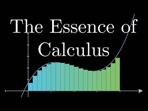
Calculus is the mathematics of change. The derivative measures how fast one quantity changes as another changes: the speed of a car, the rate at which a population grows, the extra cost of making one more item. The integral works the other way, adding up small pieces to find a total: the area under a curve, the distance travelled from a speed, the volume of a solid. These two processes undo each other, and that link is the central idea of the topic.
In the applied course, calculus is used to answer practical questions. Derivatives are used to find the dimensions of a can that uses the least metal and the time at which a reservoir is fullest; a numerical form of integration estimates the area of a field from a few measurements. At HL the topic goes much further, to motion along a line and to differential equations, which model systems where the rate of change depends on the current state, such as a cooling cup of coffee or predators and their prey.
 YouTube
How the subtopics fit together
The subtopics form three strands. The map of the topic shows each strand as a row, with the SL subtopics shaded and the HL-only subtopics dashed; an arrow means the first subtopic is used in the second.
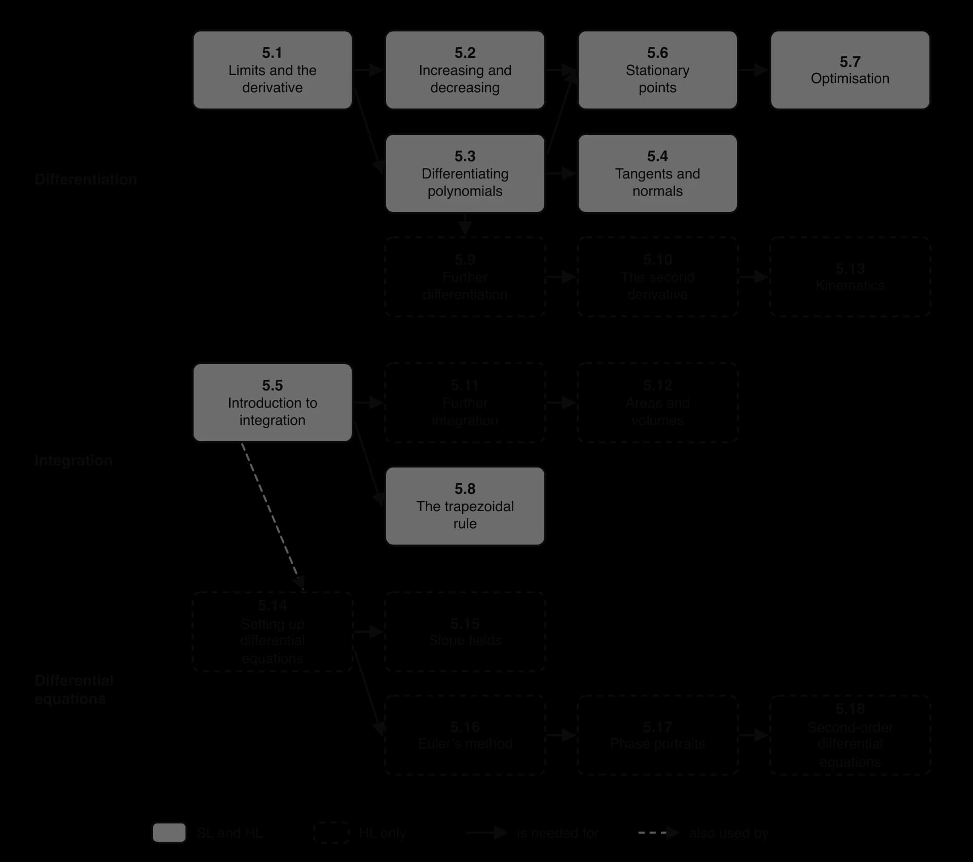
The differentiation strand starts with the derivative as the gradient of a curve, found as the limit of the gradients of shorter and shorter chords. The rule for differentiating powers of then gives derivatives quickly, and the sign of the derivative shows where a function increases or decreases. Where the derivative is zero the graph has a stationary point, and finding the largest or smallest value of a quantity in context, optimisation, is the main application at SL.
The integration strand reverses differentiation. An anti-derivative recovers a function from its gradient, and a definite integral, found with technology at SL, gives the area between a curve and the -axis. When only a table of values is known, the trapezoidal rule estimates the area from strips. At HL, more functions can be differentiated and integrated, which opens up kinematics, volumes of revolution and the differential equations strand: setting up and solving equations by separating variables, sketching slope fields, solving numerically by Euler's method, and describing coupled systems with phase portraits.
The subtopics
Subtopic | Level | What it covers |
|---|---|---|
5.1 Limits and the derivative | SL | Limits, the gradient of a curve as a limit, the derivative as a rate of change, and its notation |
5.2 Increasing and decreasing functions | SL | Where a function increases or decreases from the sign of , and reading graphs of and together |
5.3 Differentiating polynomials | SL | The derivative of for integer , including negative powers such as , term by term |
5.4 Tangents and normals | SL | Equations of the tangent and normal at a point, by hand and with technology |
5.5 Introduction to integration | SL | Anti-derivatives of integer powers (except ), finding a function from its gradient and a point, and areas by definite integrals with technology |
5.6 Stationary points | SL | Solving , local and global maximum and minimum points, and deciding their nature |
5.7 Optimisation | SL | Forming a function from a context, finding its maximum or minimum, and interpreting the result |
5.8 The trapezoidal rule | SL | Estimating areas from equally spaced values, and whether the estimate is too large or too small |
5.9 Further differentiation | HL | Derivatives of , , , , and rational powers; the chain, product and quotient rules; related rates |
5.10 The second derivative | HL | Concavity, points of inflexion and the second derivative test |
5.11 Further integration | HL | Standard integrals, integration by inspection and by substitution |
5.12 Areas and volumes | HL | Areas below the -axis, between a curve and the -axis and between two curves, and volumes of revolution about either axis |
5.13 Kinematics | HL | Displacement, velocity and acceleration along a line, and total distance travelled |
5.14 Setting up differential equations | HL | Forming differential equations from a context and solving them by separation of variables |
5.15 Slope fields | HL | Slope fields drawn with technology, sketching solution curves, and the curve on which |
5.16 Euler's method | HL | Numerical solutions of one differential equation and of coupled systems such as predator–prey models |
5.17 Phase portraits | HL | Coupled linear systems solved with eigenvalues, equilibrium points and their stability, and sketching trajectories |
5.18 Second-order differential equations | HL | Writing a second-order equation as a coupled system, then solving it by Euler's method or exactly |
Links to other topics
Calculus analyses the functions of topic 2: the maximum of a cubic model, the gradient of an exponential model at a given time, the area under a velocity–time graph. The percentage error of subtopic 1.6 measures how good a trapezoidal estimate is, and the GDC skills of subtopic 2.4 find stationary points and intersections when an equation is hard to solve by hand.
At HL the links reach further. Phase portraits classify a system by the eigenvalues of subtopic 1.15, the solutions of are the exponential models of subtopic 2.5, and the kinematics of subtopic 5.13 has a vector form in subtopic 3.12.
From the formula booklet
The entries of the mathematics: applications and interpretation formula booklet that 5 uses. Each opens in the explained booklet.
- Derivative of Topic 5: Calculus › SL and HL › SL 5.3 Derivative of
- Integral of Topic 5: Calculus › SL and HL › SL 5.5 Integral of
- Area of region enclosed by a curve and the -axis, where Topic 5: Calculus › SL and HL › SL 5.5 Area of region enclosed by a curve and the -axis, where
- The trapezoidal ruleTopic 5: Calculus › SL and HL › SL 5.8 The trapezoidal rule
- Derivative of HL onlyTopic 5: Calculus › HL only › AHL 5.9 Derivative of
- Derivative of HL onlyTopic 5: Calculus › HL only › AHL 5.9 Derivative of
- Derivative of HL onlyTopic 5: Calculus › HL only › AHL 5.9 Derivative of
- Derivative of HL onlyTopic 5: Calculus › HL only › AHL 5.9 Derivative of
- Derivative of HL onlyTopic 5: Calculus › HL only › AHL 5.9 Derivative of
- Chain ruleHL onlyTopic 5: Calculus › HL only › AHL 5.9 Chain rule
And 18 more in the formula booklet.
Carry on with 5 in Augment
With a free account, Augment remembers where you stopped and what you have practiced.