5.18 Second-order differential equations

Learning objectives

• Explain why the equations of motion of springs, dampers, circuits and falling bodies are second-order differential equations, and why they need two initial conditions.

• Show that a second-order differential equation $\ddot{x} = f(x, \dot{x}, t)$ can be written as the coupled system $\dot{x} = y$, $\dot{y} = f(x, y, t)$, and reverse the process.

• Write down the matrix $\begin{pmatrix} 0 & 1 \\ -b & -a \end{pmatrix}$ of the system for $\ddot{x} + a\dot{x} + bx = 0$

• Use Euler's method with a given step length to estimate the displacement and velocity of a second-order system, with technology.

• Find the exact solution $x = A\mathrm{e}^{\lambda_1 t} + B\mathrm{e}^{\lambda_2 t}$

• Determine whether motion is overdamped, underdamped or undamped from the eigenvalues, and sketch the matching phase portrait in the $(x, \dot{x})$ plane.

• State and interpret the long-term displacement and velocity of a system in context.

Introduction

Newton's second law says that force equals mass times acceleration, and acceleration is the second derivative of displacement. Whenever the forces on an object depend on where it is and how fast it is moving, the result is an equation containing $\ddot{x}$, $\dot{x}$ and $x$ together: a second-order differential equation. Car suspensions, vibrating bridges, swinging pendulums, falling skydivers and electric circuits are all described this way.

Such an equation looks harder than anything in subtopics 5.14–5.17, but one substitution turns it into a pair of first-order equations, the coupled systems already met. Euler's method from subtopic 5.16 then gives numerical solutions of any second-order equation, and the eigenvalue method of subtopic 5.17 gives exact solutions of the linear ones, together with a clear picture of how the motion dies away.

Second-order differential equations

Acceleration and the second derivative

The order of a differential equation is the highest derivative it contains. Every equation in subtopics 5.14–5.17 was first order. When a model is built from forces, the acceleration $\ddot{x} = \frac{\mathrm{d}^2x}{\mathrm{d}t^2}$

The dot notation of subtopic 5.13 is standard for second-order equations: $\dot{x}$ is the velocity $\frac{\mathrm{d}x}{\mathrm{d}t}$ and $\ddot{x}$

The mass–spring–damper model

A car's suspension, a door closer and the needle of a measuring instrument all contain the same three parts: a mass, a spring that pulls it back towards equilibrium, and a damper that resists its motion. The mass–spring–damper diagram shows the model with displacement $x$ measured from the equilibrium position.

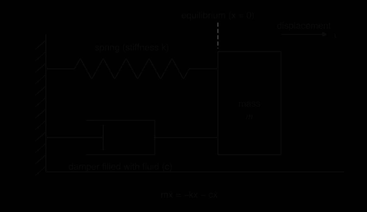
Two forces act on the mass.

• The spring pulls back towards equilibrium with a force proportional to the stretch (Hooke's law): $-kx$, where $k > 0$ is the stiffness. The minus sign means the force points opposite to the displacement.

• The damper is a piston moving through fluid. The fluid resists with a force proportional to the velocity: $-c\dot{x}$, where $c > 0$

Newton's second law, mass × acceleration = total force, gives

This has the form $\ddot{x} + a\dot{x} + bx = 0$ with $a = \frac{c}{m}$

A car's shock absorber is a damper of exactly this kind. Most are dashpots, devices that resist motion through viscous friction as a piston forces oil through small holes; the kinetic energy of a bump is turned into heat in the fluid and carried away. Without damping, the car's springs would keep the body bouncing long after every bump.

Source: Wikipedia, "Shock absorber", accessed 2026.

Other second-order models

The same mathematics appears far from cars. The table lists common second-order models and where each term comes from; each is in the form $\ddot{x} = f(x, \dot{x}, t)$.

The first three are linear with constant coefficients: $x$, $\dot{x}$ and $\ddot{x}$ appear only to the first power, multiplied by constants, with zero on the right. These are the equations that the eigenvalue method of subtopic 5.17 analyses. The falling body is non-linear (because of $\dot{x}^2$

Two initial conditions

A first-order equation needs one starting value. A second-order equation needs two, because knowing where an object is does not fix its future: a swing released from rest at a height behaves differently from one pushed from the same height. The two conditions are usually the initial displacement $x(0)$ and the initial velocity $\dot{x}(0)$. "Released from rest" means $\dot{x}(0) = 0$

A proposed solution can always be checked by differentiating twice and substituting, as in subtopic 5.14.

Writing a second-order equation as a coupled system

The substitution y = ẋ

The key idea is to treat the velocity as a second unknown. Define $y = \dot{x}$. Differentiating once more gives $\dot{y} = \ddot{x}$. So the single equation $\ddot{x} = f(x, \dot{x}, t)$

The first equation is just the definition of $y$. The second is the original equation with $\ddot{x}$ written as $\dot{y}$ and $\dot{x}$

Nothing is lost in the rewriting: a solution $x(t)$ of the second-order equation gives a solution $(x, \dot{x})$ of the system, and a solution $(x, y)$ of the system gives a solution $x$

For the linear equation $\ddot{x} + a\dot{x} + bx = 0$, solving for $\ddot{x}$

The first row is always $(0, 1)$, because $\dot{x} = 0x + 1y$. The second row holds the coefficients with their signs changed, in the order $x$ then $y$

Non-linear and forced equations

The substitution works for any equation that can be solved for $\ddot{x}$, linear or not. Only the second equation changes.

Forced and non-linear systems cannot be written as $\dot{\boldsymbol{x}} = M\boldsymbol{x}$, so the eigenvalue method does not apply to them; Euler's method does.

The reverse process also matters: a coupled system with $\dot{x} = y$ can be turned back into one second-order equation by differentiating the first equation and substituting the second.

The sign of each coefficient also needs care, because the terms of the equation change sides when it is solved for $\ddot{x}$.

Numerical solutions with Euler's method

The coupled Euler scheme

Euler's method for a coupled system (subtopic 5.16) steps both variables forward together, using the values at the start of each step. With step length $h$:

For a second-order equation reduced with $y = \dot{x}$, $f_1 = y$, so the scheme becomes

In words: the new displacement is the old displacement plus velocity × time step, and the new velocity is the old velocity plus acceleration × time step. Both updates use the old values $x_n$, $y_n$, $t_n$

The value 7 m s⁻¹ is far below a real skydiver's terminal speed, because the drag constant 0.2 is invented to keep the numbers simple. A real skydiver falling face down has a terminal speed of about 55 m s⁻¹, which corresponds to a much smaller constant ($\frac{9.8}{55^2} \approx 0.003$). The model still shows the mechanism correctly. Drag grows with speed until it balances the weight, so the velocity approaches the terminal velocity without ever passing it. Subtopic 5.13 describes a record-breaking real jump in which the speed rose and then fell as the air thickened.

Source: Wikipedia, "Terminal velocity", accessed 2026.

Setting up the technology

Euler values are generated with technology, not by hand. Three set-ups are common.

• Spreadsheet: columns for $t$, $x$ and $y$; the first row holds 0, $x(0)$ and $\dot{x}(0)$

The number of steps is $\frac{\text{final } t - \text{initial } t}{h}$: from 0 to 1 with $h = 0.1$ is 10 steps. For the write-up, record the recurrences with the actual numbers in them, the step length, and the final values; a full table is not needed.

A forced equation and its long-term behaviour

When a forcing term pushes the system, it does not settle at rest, but it may settle into a steady pattern that Euler's method shows clearly.

The long-term velocity can be understood without the exact solution. The forcing term $8t + 6$ grows steadily. Once the transient motion has died away, the particle moves so that $8x$ keeps pace with $8t$, which means $x$ grows like $t$ and the velocity is 1.

Exact solutions of ẍ + aẋ + bx = 0

The matrix, its eigenvalues and the auxiliary equation

The system for $\ddot{x} + a\dot{x} + bx = 0$ has matrix $M = \begin{pmatrix} 0 & 1 \\ -b & -a \end{pmatrix}$

This quadratic can be written straight from the differential equation: replace $\ddot{x}$ by $\lambda^2$, $\dot{x}$ by $\lambda$

The eigenvectors and the solution for x

For an eigenvalue $\lambda$, the first row of $M - \lambda I$ is $(-\lambda, 1)$, so an eigenvector $\begin{pmatrix} p \\ q \end{pmatrix}$

which makes sense: along this direction the velocity $y$ is $\lambda$ times the displacement $x$, exactly as for $x = \mathrm{e}^{\lambda t}$, whose derivative is $\lambda x$

With real distinct eigenvalues $\lambda_1$ and $\lambda_2$, the general solution of subtopic 5.17 is

and its first component is the displacement:

The constants come from the two initial conditions: $x(0) = A + B$ and $\dot{x}(0) = A\lambda_1 + B\lambda_2$

Using the GDC

The algebra in this method is short, and the GDC is used at two points: solving the auxiliary equation and analysing the final $x(t)$.

1. Solve $\lambda^2 + a\lambda + b = 0$ with the polynomial root finder (on a TI-84 Plus CE: APPS → PlySmlt2 → POLYNOMIAL ROOT FINDER; on a Casio fx-CG50: MENU → Equation → POLY). Complex roots show at once that the motion is underdamped.

2. Solve the two equations for $A$ and $B$

Write down the auxiliary equation, its roots, the two equations for the constants and the equation solved for a time; a bare decimal with no equation behind it shows no method.

YouTube

Case study: settling after a bump

The shock-absorber equation $\ddot{x} + 3.5\dot{x} + 1.5x = 0$ is a simple model of a damped car suspension. Suppose a bump compresses the spring so that the body is displaced 6 cm from equilibrium, and the motion starts from rest: $x(0) = 6$

The auxiliary equation is $\lambda^2 + 3.5\lambda + 1.5 = 0$, which factorises as $(\lambda + 0.5)(\lambda + 3) = 0$

The initial conditions give two equations for the constants:

From the second equation $A = -6B$, so $-5B = 6$, giving $B = -1.2$ and $A = 7.2$

Both exponentials decay, so the body returns to equilibrium without ever overshooting: $x$ stays positive for all $t$. The fast term $-1.2\mathrm{e}^{-3t}$ matters only in the first second, where it makes the motion start gently from rest; after that the slow term $7.2\mathrm{e}^{-0.5t}$

Euler's method with $h = 0.1$ gives a check on the exact solution. The Euler estimates lie close to the exact curve: at $t = 1$, Euler gives $x \approx 4.277$ cm against the exact 4.307 cm, an error of about 0.7%. Halving the step to $h = 0.05$

The coefficients of the model, the initial displacement and the 0.5 cm threshold are hypothetical.

Damping and long-term behaviour

Three kinds of motion

The roots of $\lambda^2 + a\lambda + b = 0$ depend on the sign of the discriminant $a^2 - 4b$. For a mass on a spring with damping ($a > 0$

When the damping is strong ($a^2 > 4b$), the eigenvalues are real, distinct and both negative, because their sum is $-a < 0$ and their product is $b > 0$. The displacement is a sum of two decaying exponentials, so the mass returns to equilibrium without oscillating.

When the damping is weaker ($a^2 < 4b$), the eigenvalues are complex, $\alpha \pm \beta\mathrm{i}$, with real part $\alpha = -\frac{a}{2} < 0$

For $\ddot{x} + \dot{x} + 4.25x = 0$, $\lambda = \frac{-1 \pm \sqrt{1 - 17}}{2} = -0.5 \pm 2\mathrm{i}$

With no damping at all ($a = 0$), the eigenvalues are purely imaginary and nothing removes energy, so the oscillation never dies away.

The boundary case $a^2 = 4b$, called critical damping, gives a repeated eigenvalue and the fastest return to equilibrium without overshoot. A repeated eigenvalue needs a different form of solution, outside the method for distinct eigenvalues.

Phase portraits in the (x, ẋ) plane

Because the system variables are $x$ and $y = \dot{x}$, the phase plane of a second-order equation has displacement on the horizontal axis and velocity on the vertical axis. The three damping cases give three of the portraits of subtopic 5.17.

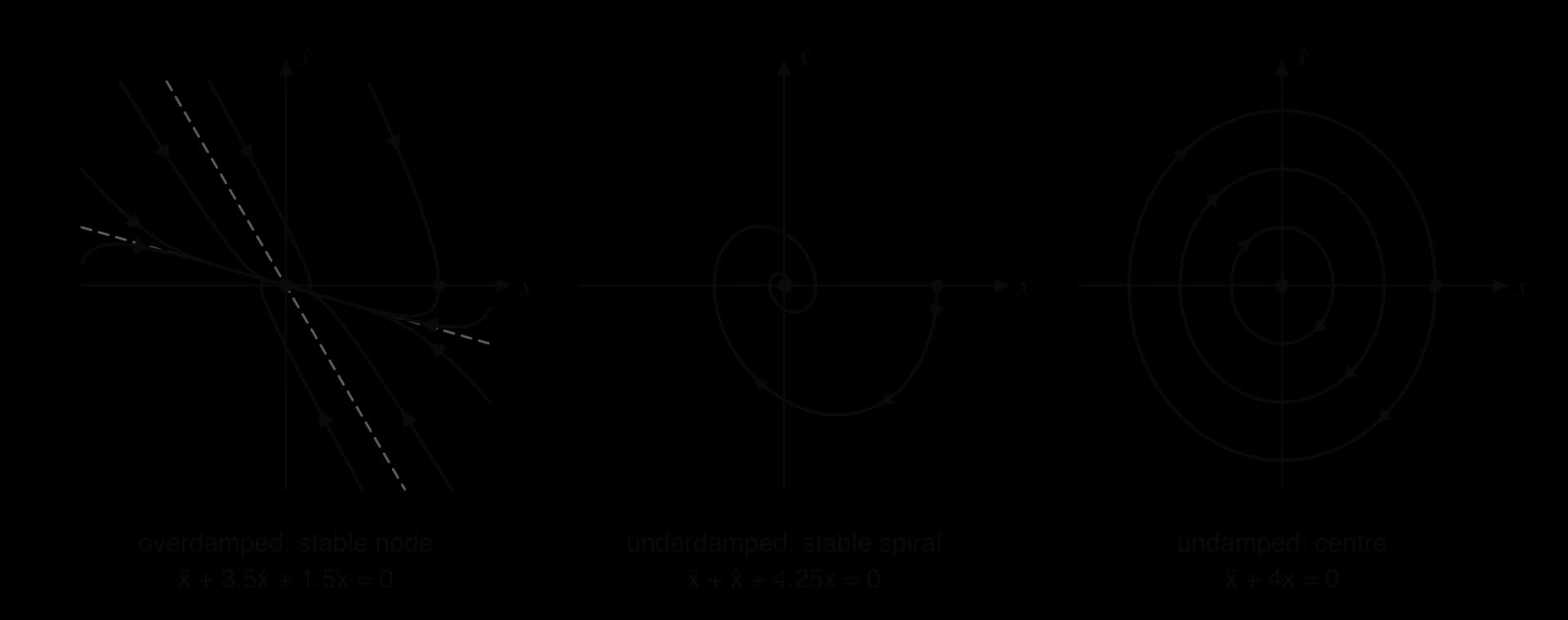
Two features are true of every $(x, \dot{x})$ phase portrait.

• Motion is to the right in the upper half-plane and to the left in the lower half-plane, because $\dot{x} = y$: positive velocity means increasing displacement. Trajectories therefore cross the $x$-axis vertically.

• Spirals and centres turn clockwise when $b > 0$. On the positive $x$

For the overdamped shock absorber, the eigenvector lines are $\dot{x} = -0.5x$ and $\dot{x} = -3x$. Trajectories enter the origin along $\dot{x} = -0.5x$

Simple harmonic motion

The undamped equation is important enough to have its own name. Writing $b = \omega^2$:

The matrix $\begin{pmatrix} 0 & 1 \\ -\omega^2 & 0 \end{pmatrix}$ has trace 0 and determinant $\omega^2$

A mass on a frictionless spring has $\omega^2 = \frac{k}{m}$, and a pendulum of length $L$ swinging through small angles has $\omega^2 = \frac{g}{L}$

Long-term velocity and displacement

For the unforced equation $\ddot{x} + a\dot{x} + bx = 0$ the long-term behaviour follows from the eigenvalues alone.

So when both eigenvalues are negative, the long-term velocity is 0, with no solving needed. With a forcing term or a non-linear equation, set $\ddot{x} = 0$ (constant velocity) or read the limit from a long Euler run. For $\ddot{x} + 6\dot{x} + 8x = 8t + 6$

YouTube

Exam focus

Second-order equations are examined on HL Paper 1 (4–6 marks, usually rewriting as a system and a short Euler calculation) and Paper 2 (10–17 marks, usually a context such as a shock absorber, a pollutant or a particle, combining the eigenvalue method with interpretation). The equation is always given. Typical command terms are show that (the system or the equation), write down (the matrix), find (eigenvalues, the exact solution, an Euler estimate), sketch ($x$ against $t$, with a maximum labelled), state (the long-term velocity) and write down a reason in context.

What to write: the explicit link $y = \dot{x} \Rightarrow \dot{y} = \ddot{x}$; the matrix; the characteristic equation and eigenvalues; the general solution with $x = \ldots$

The state in part (e) means no working is expected: two negative eigenvalues mean the system comes to rest, so the velocity tends to 0. Solving the system again earns nothing and wastes time. Part (g) can also be answered by continuing the Euler table, which settles at $x = 2.00$.

Eigenvalue errors are costly here as in subtopic 1.15: a wrong eigenvalue makes the later parts impossible to follow through. Check the eigenvalues against the auxiliary equation by sum and product ($\lambda_1 + \lambda_2 = -a$, $\lambda_1\lambda_2 = b$

Practice questions

1. Write $\ddot{x} + 4\dot{x} + 3x = 0$ as a coupled first-order system and write down its matrix. [3]

2. Show that $x = 3\mathrm{e}^{-t} - \mathrm{e}^{-3t}$

Summary

• A second-order differential equation contains $\ddot{x}$; models built from forces (springs, dampers, drag, circuits) give such equations, and each needs two initial conditions, $x(0)$ and $\dot{x}(0)$.

• The substitution $y = \dot{x}$

Self-check

• To do:

  I can explain where each term of $m\ddot{x} = -kx - c\dot{x}$ comes from.

• To do:

  I can check that a given function solves a second-order equation by differentiating twice.

• To do:

  I can write $\ddot{x} = f(x, \dot{x}, t)$