5.8 The trapezoidal rule

Introduction

Many areas in the real world have no formula. The surface of a lake, the cross-section of a river, the region under a speed–time graph recorded by a sensor every ten seconds: each usually comes as a shape on a map or as a table of measurements, rarely as a neat function. Even when a function is known, its integral may be impossible to find by hand. The trapezoidal rule gives an estimate of such an area by cutting it into thin vertical strips and replacing each strip by a trapezoid, a shape whose area is easy to calculate.

Surveyors, engineers and scientists use the same idea. Hydrologists find the flow of a river from depths measured at equal spacings across it, and naval architects estimate the volume of a ship's hull from widths measured at equal intervals along it. The method is a first example of numerical integration, which replaces an exact calculation by an approximate one built from a finite set of values.

Why areas need to be approximated

Subtopic 5.5, Introduction to integration, finds the area under a curve $y = f(x)$ between $x = a$ and $x = b$ as a definite integral.

That calculation needs a formula for $y$ and a way to evaluate the integral. In practice at least one of these is often missing.

• The data are a table, not a function. A speedometer reading every 10 seconds, a depth sounding every metre across a river, or a width measured every 200 metres along a lake gives values at separate points only. Nothing is known about the curve between them.

• The function cannot be integrated by hand. Functions such as $y = \sqrt{1 + x^3}$ or $y = 2^{-x^2}$ have no anti-derivative that can be written with the usual functions, so their integrals must be estimated.

• A quick check is wanted. Even when an exact method exists, an independent estimate shows whether a calculator answer is reasonable.

In each case the area is replaced by shapes whose areas are known. The simplest choice is a set of rectangles, but rectangles step up and down and miss every slope of the curve. The top edge of each trapezoid joins two points on the curve with a straight line, so a set of trapezoids follows a sloping curve far more closely. The Khan Academy video on trapezoidal sums builds this comparison step by step.

The area of a trapezoid

A trapezoid (called a trapezium in British English) is a four-sided shape with one pair of parallel sides. In the trapezoidal rule each trapezoid stands upright: its two parallel sides are vertical and its base lies on the $x$-axis.

If the parallel sides have lengths $p$ and $q$ and the distance between them is $h$, the area is the mean of the parallel sides multiplied by the distance between them.

The formula is easy to justify. Two copies of the same trapezoid, one turned upside down, fit together into a parallelogram of base $p + q$ and height $h$. The parallelogram has area $(p + q)h$, so one trapezoid has half of it. Equivalently, the trapezoid has the same area as a rectangle of width $h$ whose height is the average of $p$ and $q$.

The trapezoidal rule

Strips, the strip width and ordinates

To estimate $\int_a^b y\,\mathrm{d}x$, the interval from $x = a$ to $x = b$ is divided into $n$ strips of equal width. The width of each strip is the length of the interval divided by the number of strips.

The edges of the strips are at $x_0 = a$, $x_1 = a + h$, $x_2 = a + 2h$, and so on up to $x_n = a + nh = b$. The height of the curve at each edge is called an ordinate.

Counting the edges needs care. A fence with 4 gaps has 5 posts, and in the same way $n$ strips have $n + 1$ edges, so they need $n + 1$ ordinates. Four strips use the five ordinates $y_0, y_1, y_2, y_3, y_4$; a table with seven $y$-values gives six strips.

Deriving the rule

The diagram of four trapezoidal strips under a curve shows the idea. Each strip from $x_{k-1}$ to $x_k$ is replaced by a trapezoid with parallel sides $y_{k-1}$ and $y_k$ and width $h$, so its area is $\frac{1}{2}h(y_{k-1} + y_k)$.

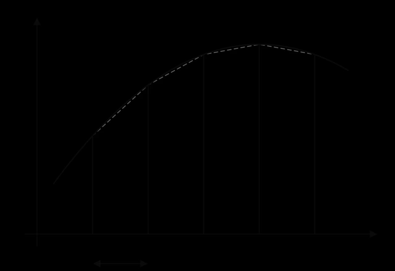
Adding the four trapezoids gives the estimate, and collecting terms shows the pattern.

The first and last ordinates appear once each, because each forms a side of only one trapezoid. Every ordinate in between is the right-hand side of one trapezoid and the left-hand side of the next, so it is counted twice. The same reasoning works for any number of strips.

In words: add the first and last ordinates, add twice the sum of all the others, and multiply by half the strip width. An equivalent reading is that the estimate equals the width $b - a$ multiplied by a weighted average of the heights, in which the end ordinates carry half the weight of the middle ones.

Applying the rule to a function

When $y$ is given as a function, the ordinates are found by substituting each strip edge into the function. A small table keeps the work organised and makes it easy to see which values are doubled.

The graph of $y = 6 + 4x - x^2$ with its four chords shows why the estimate in the worked example came out too small. The curve bulges upwards between every pair of neighbouring ordinates, so each chord runs just beneath the curve and each trapezoid misses a thin sliver of area.

Using the rule with a table of data

Most real uses of the trapezoidal rule start from measurements, not a formula. The method is the same: the strip width is the equal spacing of the $x$-values, the first and last measurements are the end ordinates, and everything in between is doubled.

The table gives values of a function $y = f(x)$ at equally spaced values of $x$.

Distance from a table of speeds

The area under a speed–time graph is the distance travelled, because over a short time interval distance is speed multiplied by time, which is the area of a thin strip under the graph. A table of speeds recorded at equal time intervals can therefore be turned into a distance with the trapezoidal rule. The units of the area are the units of $y$ multiplied by the units of $x$: metres per second multiplied by seconds gives metres.

A car pulls away from traffic lights. Its speed $v$ metres per second is recorded every 10 seconds for one minute.

Cross-sections and river flow

The area of a cross-section is found the same way, with the distance across as $x$ and a depth or a height as $y$. Hydrologists measure the flow of a river by wading or boating across it, recording the depth at equal spacings. The cross-sectional area multiplied by the mean speed of the water gives the discharge, the volume of water passing a point each second, in cubic metres per second. The worked example uses hypothetical soundings.

A stream is 12 m wide. Its depth $d$ metres is measured every 2 m across it, starting at one bank.

Strips of unequal width

The trapezoidal rule in the formula needs strips of equal width, because the common factor $\frac{1}{2}h$ is taken outside the bracket. When measurements are taken at unequal spacings, each strip is a trapezoid with its own width, and the areas are added one by one with $\frac{1}{2}(p + q)h$. If some neighbouring strips do share a width, the rule can still be applied to that group.

A gardener measures the width of a flower border at several points along a straight path that forms one edge of it. The border meets the path in a point at both ends.

The first two strips in the worked example share $h = 2$, and the last two share $h = 3$, so the rule could be applied to each pair separately: $\frac{1}{2} \times 2 \times (0 + 2.5 + 2 \times 1.8) + \frac{1}{2} \times 3 \times (2.5 + 0 + 2 \times 2.2) = 6.1 + 10.35 = 16.45$. The two methods always agree, because the rule is only a shortcut for adding trapezoids.

Working backwards from an estimate

Because the rule is a single equation, a missing ordinate or strip width can be found when the estimate is given. Substituting everything that is known and solving the resulting linear equation gives the unknown value.

The table gives values of $y = g(x)$.

Using technology

The GDC has no button for the trapezoidal rule, but it shortens the arithmetic and gives the accurate value of the integral that an estimate is compared with. The substituted formula is still written out in full, because it shows the method and lets each ordinate be checked.

Calculating the estimate with lists

1. Enter the ordinates in one list and the weights 1, 2, 2, …, 2, 1 in a second list. On a TI-84 Plus CE, use STAT → EDIT and type them into L1 and L2.

2. Multiply the lists term by term and add the results: on a TI-84 Plus CE, sum(L1*L2), with sum( found under 2nd LIST → MATH.

3. Multiply the result by $\frac{1}{2}h$.

A spreadsheet works the same way: one column of ordinates, one column of weights, a column of their products, then the total multiplied by $\frac{h}{2}$. For a function, a third column computing $f(x)$ from the $x$-values avoids substitution errors.

Comparing with the definite integral

When the function is known, the GDC's numerical integration finds $\int_a^b f(x)\,\mathrm{d}x$ to many decimal places: on a TI-84 Plus CE use fnInt( from the MATH menu, and on a Casio fx-CG50 use Run-Matrix → OPTN → CALC → ∫dx; from a graph, most GDCs shade the area and display the integral directly. This value is treated as the exact value against which the estimate is judged. The size of the error is usually given as a percentage error.

Here $v_A$ is the trapezoidal estimate and $v_E$ the value of the integral.

Accuracy of the estimate

Overestimates and underestimates

Every trapezoidal estimate differs a little from the true area, unless the curve happens to be made of straight line segments joining the ordinates. Knowing whether the estimate is too large or too small turns a single number into a bound on the true value, in the same way as upper and lower bounds in subtopic 1.6.

An estimate of 783 m for a distance that is truly 790 m is an underestimate; an estimate of 30.5 for an integral equal to 30.06 is an overestimate.

Concavity and the direction of the error

The direction of the error depends only on where the chords lie compared with the curve. If every chord lies on or above the curve, every trapezoid contains its strip of area plus a little extra, so the estimate is too large. If every chord lies on or under the curve, every trapezoid misses a little of its strip, so the estimate is too small. The position of the chords is decided by the way the curve bends.

A concave-up curve has the shape of the inside of a bowl: it would hold water. Exponential growth curves, $y = \frac{1}{x}$ for $x > 0$ and the cost of producing ever more units of a product often have this shape.

A concave-down curve has the shape of an arch or an upturned bowl. Speeds that rise quickly and then level off, and the height of a thrown ball, have this shape. The side-by-side diagram of the two cases shows the gaps that make up the error.

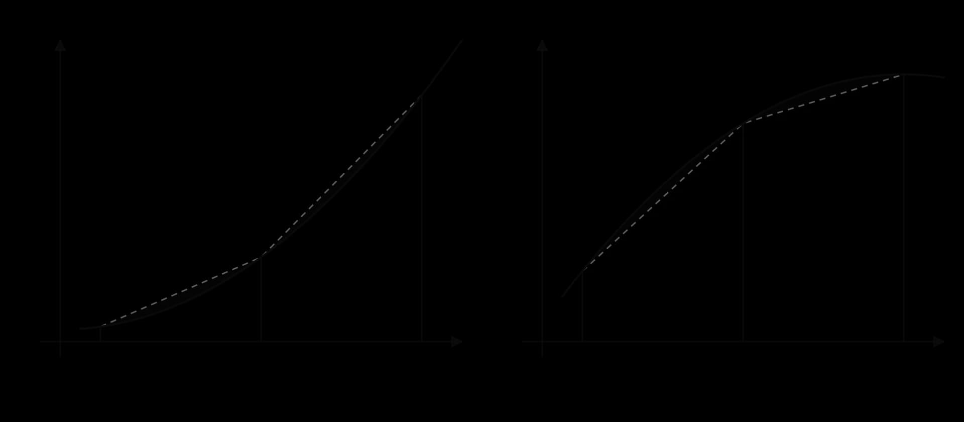
The two results are summarised in a short table.

The direction of the error depends only on the bend of the curve, whether the curve is rising or falling. A decreasing curve that bends upwards, such as $y = \frac{1}{x}$ for $x > 0$, still gives an overestimate.

Curves that change concavity

Many real curves bend one way and then the other, like the S-shape of a population that grows slowly, then quickly, then slowly again. On the concave-up part the chords lie above the curve and on the concave-down part they lie below it, so some errors are positive and some negative. They partly cancel, and the total estimate may be too large, too small or very nearly exact. In that case the shape of the graph does not settle the question; only a comparison with a more accurate value, such as the GDC integral or an estimate with many more strips, can decide it.

More strips, a better estimate

Thinner strips follow the curve more closely, so the gaps between the chords and the curve shrink. The table shows the effect for $\int_0^4 3 \times 1.5^x\,\mathrm{d}x = 30.0580\ldots$ as the number of strips doubles.

Every estimate is an overestimate, as the concave-up shape predicts, and each one is closer than the last. The errors also follow a pattern: each time the strip width halves, the error falls to about a quarter. The error of the trapezoidal rule is roughly proportional to $h^2$, so ten times as many strips gives about a hundred times the accuracy.

With a table of measurements, the number of strips is fixed by the data, so the only way to improve the estimate is to take more measurements, closer together. Where the curve bends sharply, such as near the ends of a lake or where a speed changes suddenly, extra measurements improve the estimate most.

Case study: the area of Lake Bled

Lake Bled is a lake of glacial and tectonic origin in the Julian Alps of north-western Slovenia, about 2,120 m long and 1,380 m wide at its longest and widest lines, with a small island near its western end. Its outline is irregular, with no formula, so its area is a natural problem for the trapezoidal rule. The method is the surveyor's offset method: draw a straight baseline along the length of the lake, then measure the width of the lake at right angles to the baseline at equal intervals.

The widths were measured north–south across the lake on its OpenStreetMap outline, at 11 equally spaced points from the western tip to the eastern tip, and rounded to the nearest 10 m. The two tips touch the baseline at single points, so the end widths are 0.

Source: widths measured from the OpenStreetMap outline of Lake Bled (© OpenStreetMap contributors), 2026; published dimensions from Wikipedia, "Lake Bled", 2026.

There are 10 strips, so $h = \frac{2040}{10} = 204$ m. The end widths are both 0 and the nine middle widths add up to 6,790 m.

The estimate is about 1.39 km² (1 km² = 1,000,000 m²). The published area of the lake is 1.45 km².

Ten widths give the area to within about 5%, with only a ruler and a map. The estimate is too small, and comparing each trapezoid with the true area of its strip shows where the shortfall comes from. The largest gaps are in the second strip from the west, where the shore swings out quickly towards the widest part of the lake, and in the strip at the eastern tip, where the width rises fast from 0 and then levels off. In both places the graph of width against distance is concave down, so the chords run inside the true outline and cut off area. In the middle of the lake the width rises and falls irregularly, some chords lie on each side of the curve, and the errors partly cancel. Measuring every 102 m instead (20 strips) gives about 1.43 km², closer to the published value, as the pattern in the table of strip numbers predicts.

The calculation has other limitations. The widths are rounded to the nearest 10 m, and the map outline itself is an approximation; the area of a lake also changes slightly with its water level. The width through the island includes the island, about a hectare of land. These sources of error are smaller than the effect of the strip width here, which is why surveyors measure offsets more closely where a boundary curves sharply.

Extension: Simpson's rule

Simpson's rule is an extension for interest. The trapezoidal rule joins neighbouring points with straight lines. A natural improvement joins them with curves instead: Simpson's rule fits a parabola through each set of three neighbouring points. It is named after the English mathematician Thomas Simpson (1710–1761).

For $\int_0^4 3 \times 1.5^x\,\mathrm{d}x$ with 4 strips, Simpson's rule gives $\frac{1}{3}\left(18.1875 + 4(4.5 + 10.125) + 2(6.75)\right) = 30.0625$, within 0.02% of the true value 30.058, against 1.37% for the trapezoidal rule with the same five ordinates. Simpson's rule is exact for every quadratic and cubic function, so it would give the exact area under $y = 6 + 4x - x^2$.

Exam focus

The trapezoidal rule appears on Paper 1 as a short question of 3–4 marks, and on Paper 2 as the first part of a longer question about a shape, a region in a design or a table of measurements. The usual command terms are use (the trapezoidal rule), estimate, find and write down (the value of $h$). Questions often go on to ask for the exact area by integration with the GDC, the percentage error of the estimate, or the area of a related region, and they may ask the student to explain or justify whether the estimate is too large or too small.

Markschemes award (A1) for the value of $h$ seen, (M1) for a correct substitution into the rule, and A1 for the answer. A zero end ordinate may be left out of the working. An over- or underestimate earns its reasoning mark only with a reason about the shape of the curve.

The most common lost mark is the strip width. Examiners report many wrong values of $h$, usually from dividing by the number of values in the table instead of the number of strips.

When a question asks whether an estimate is too large or too small, a calculation alone is not a reason. Comparing the estimate with a known exact value shows that it is an underestimate, but the mark for explain or justify needs why: the shape of the curve and the position of the chords.

Practice questions

1. The interval $2 \le x \le 5$ is divided into 6 strips of equal width. Write down the strip width and the number of ordinates needed. [2]

2. Use the trapezoidal rule to estimate $\int_0^8 f(x)\,\mathrm{d}x$ from the table. [3]

3. (a) Use the trapezoidal rule with 3 strips to estimate $\int_0^3 (x^2 + 2)\,\mathrm{d}x$. (b) Find the exact value of the integral using technology. (c) Calculate the percentage error. [6]

4. A drone takes off vertically. Its speed is recorded every 5 seconds: 0, 4.8, 8.6, 10.2, 10.9 and 11.0 m s⁻¹ at $t = 0, 5, 10, 15, 20, 25$. Estimate the distance it travels in the first 25 seconds. [3]

5. The values of $y = h(x)$ at $x = 0, 0.5, 1, 1.5, 2$ are 2, 3, $p$, 4 and 2. The trapezoidal rule gives $\int_0^2 h(x)\,\mathrm{d}x \approx 6.25$

6. A canal is 10 m wide. Its depth is measured every 2 m across it: 0, 0.6, 1.1, 1.3, 0.7 and 0 m. (a) Estimate the area of the cross-section. (b) The water flows at a mean speed of 0.4 m s⁻¹. Estimate the volume of water passing a point each minute. [5]

7. Let $f(x) = \frac{20}{x}$. (a) Use the trapezoidal rule with 4 strips to estimate $\int_1^5 f(x)\,\mathrm{d}x$

8. The top edge of a window is modelled by $y = -0.1x^3 + 0.9x^2 - 1.5x + 4$ for $0 \le x \le 4$

Summary

• The trapezoidal rule estimates $\int_a^b y\,\mathrm{d}x$ by replacing the curve with straight chords and adding the areas of the trapezoids under them.

• $\int_a^b y\,\mathrm{d}x \approx \frac{1}{2}h\left((y_0 + y_n) + 2(y_1 + \cdots + y_{n-1})\right)$, with $h = \frac{b - a}{n}$ (in the formula booklet).

• $n$ strips need $n + 1$ ordinates; the end ordinates are used once and every middle ordinate twice, because it is shared by two trapezoids.

• From a table, $h$ is the equal spacing of the $x$-values; from a function, the ordinates are found by substitution.

• The area under a rate graph is an accumulated total: speed × time gives distance, depth × width gives a cross-section.

• Strips of unequal width are added one by one with $\frac{1}{2}(p + q)h$.

• The GDC's definite integral gives the value an estimate is compared with; the percentage error measures the accuracy.

• A concave-up curve gives an overestimate and a concave-down curve an underestimate; a curve that changes concavity needs a numerical comparison.

• More strips give a better estimate: halving $h$ cuts the error to about a quarter.

Self-check

• To do:

  I can find the strip width $h$ from an interval and a number of strips, or from a table.

• To do:

  I can say how many ordinates a given number of strips needs.

• To do:

  I can explain why the middle ordinates are doubled and the end ordinates are not.

• To do:

  I can apply the trapezoidal rule to a function, making a table of ordinates first.

• To do:

  I can apply the trapezoidal rule to a table of measurements, including zero end values.

• To do:

  I can estimate a distance from a table of speeds and give the answer with units.

• To do:

  I can add trapezoids of unequal width one at a time.

• To do:

  I can find a missing ordinate when the trapezoidal estimate is given.

• To do:

  I can use the GDC to find the definite integral and the percentage error of an estimate.

• To do:

  I can identify concave-up and concave-down curves and the position of their chords.

• To do:

  I can justify whether an estimate is an overestimate or an underestimate with a reason about the curve's shape.

• To do:

  I can explain why a curve that changes concavity needs a numerical check.

• To do:

  I can explain how increasing the number of strips changes the accuracy of the estimate.

• To do:

  I can write down the substituted formula and the integral in the form a markscheme rewards.

where $h(x)$ is the height of the mound, in metres, at a horizontal distance of $x$ metres from one end of the cross-section. The cross-section is the region between the graph of $h$, the $x$-axis and the lines $x = 0$ and $x = 12$.

1. (a)

   Complete the following table.

   $x$	0	2	4	6	8	10	12
   $h(x)$	1	2.2		7.48	8.68		1

   [2]2 marks

   Markscheme (a)

   $h(4) = 4.84$ A1

   $h(10) = 7$ A1

   [2 marks]

2. (b)

   Use the trapezoidal rule with the values in the table to estimate the area of the cross-section.

   [3]3 marks

   Markscheme (b)

   $\dfrac{2}{2}\left[1 + 1 + 2(2.2 + 4.84 + 7.48 + 8.68 + 7)\right]$

3. (c)

   Write down an integral for the exact area of the cross-section, and hence find this area.

   [2]2 marks

   Markscheme (c)

   $\displaystyle\int_{0}^{12} \left(-0.03x^{3} + 0.36x^{2} + 1\right) \mathrm{d}x$

4. (d)

   Calculate the percentage error in the estimate found in part (b).

   [2]2 marks

   Markscheme (d)

   $\left|\dfrac{62.4 - 63.84}{63.84}\right| \times 100\%$

5. (e)

   Priya repeats the estimate using the trapezoidal rule with 12 intervals, and obtains 63.48 m².

   Find the percentage error in this estimate, and comment on the effect of using more intervals.

   [2]2 marks

   Markscheme (e)

   $\left|\dfrac{63.48 - 63.84}{63.84}\right| \times 100 = 0.564\%$

6. (f)

   The mound is 30 m long and has the same cross-section along its whole length.

   Find the volume of earth needed to build the mound.

   [2]2 marks

   Markscheme (f)

   $63.84 \times 30$ (M1)

   $1915.2$ (m³) $(1920)$ A1

   Note: Follow through from part (c).

   [2 marks]

7. (g)

   Earth costs 18.40 euros (EUR) per m³. Priya's budget for earth is 35 000 EUR.

   Determine whether Priya's budget is enough. Justify your answer.

   [3]3 marks

   Markscheme (g)

   $1915.2 \times 18.40$ (M1)

   $35\,239.68$ (EUR) A1

   $35\,239.68 > 35\,000$, so the budget is not enough

(b) The end ordinates are 2.4 and 2.0; the middle ones are 3.1, 3.9, 4.2 and 3.6.

The estimate is 25.5.

So $k = 6.5$. Check: $0.25 \times (9 + 2 \times 23.5) = 0.25 \times 56 = 14$.

The estimate is 30.5 (3 s.f.).

(b) The graph of $g$ is concave up, so each chord lies above the curve and each trapezoid includes some area that is not under the curve. The estimate is an overestimate.

(c) The GDC gives $\int_0^4 3 \times 1.5^x\,\mathrm{d}x = 30.0580\ldots$

The percentage error is 1.37%. The overestimate in part (b) is confirmed: $30.47 > 30.06$.

$= 69\text{ m}^2$ A1

(c) (i) $\int_0^{10} (5 + 1.4x - 0.15x^2)\,\mathrm{d}x$ A1A1

Award A1 for the correct limits and A1 for the integrand with $\mathrm{d}x$.

(ii) $70\text{ m}^2$ A1

(d) $\left|\frac{69 - 70}{70}\right| \times 100\%$ (M1)

$= 1.43\%$ $(1.428571\ldots\%)$ A1

(e) The curve is concave down (it bends downwards), so the chords of the trapezoids lie below the curve R1

the trapezoids miss some of the area under the curve, so the trapezoidal rule underestimates the area A1

Do not award R0A1.

Total [10]

$62.4$ (m²) A1

Note: Award the method mark for an attempt to use the trapezoidal rule with $h = 2$, and the next mark for correct substitution. Follow through from part (a).

[3 marks]

$63.84$ (m²) $(63.8)$ A1

[2 marks]

$2.26\%$ $(2.25563\ldots)$ A1

Note: Follow through from parts (b) and (c).

[2 marks]

using more (narrower) intervals reduces the percentage error (gives a more accurate estimate) R1

[2 marks]

Note: Follow through from part (f). Do not award the reasoning mark without a comparison.

[3 marks]

• roof

Find the value of $p$ and the value of $q$.

[2]2 marks