Augment Education
  • Blog
Log inStart free
augment

Augment Education

IB Diploma revision built around the syllabus.

contact@augment-education.com

Product

  • Features
  • Question bank
  • Quick fire
  • Worksheets
  • Flashcards
  • Notes
  • Subjects
  • What's new

Learn

  • IB guide
  • Booklets, explained
  • Blog
  • Free tools
  • Grade calculator
  • Subject checker

Company

  • About
  • Help
  • For parents
  • For teachers
  • Student stories
  • Comparisons

Augment Education is developed independently of the International Baccalaureate Organization and is not endorsed by it. “IB” and “International Baccalaureate” are its trademarks.

© 2026 Augment Education. All rights reserved.

PrivacyTerms
  1. Subjects
  2. Maths AI
  3. 5 Calculus
  4. 5.15 Slope fields

5.15 Slope fields

Build and read slope fields, calculate gradients from a differential equation, sketch solution curves through given points, and use the curve where dy/dx = 0 to locate maxima and minima of solutions.

  • IB Mathematics: Applications and Interpretation
  • Part of 5 Calculus
  • HL only

Key terms introduced here

Each is in the Maths AI glossary, with every other term in the subject.

Autonomous differential equation

A first-order differential equation dydx=f(y)\frac{\mathrm{d}y}{\mathrm{d}x} = f(y)dxdy​=f(y) whose right-hand side depends only on the unknown yyy and not on the independent variable.

Isocline

A curve along which every solution of a differential equation dydx=f(x,y)\frac{\mathrm{d}y}{\mathrm{d}x} = f(x, y)dxdy​=f(x,y) has the same gradient ccc; its equation is f(x,y)=cf(x, y) = cf(x,y)=c.

Nullcline

The isocline on which dydx=0\frac{\mathrm{d}y}{\mathrm{d}x} = 0dxdy​=0, with equation f(x,y)=0f(x, y) = 0f(x,y)=0; every local maximum and local minimum of a solution curve lies on it.

Slope field

A diagram of a first-order differential equation dydx=f(x,y)\frac{\mathrm{d}y}{\mathrm{d}x} = f(x, y)dxdy​=f(x,y) made of short line segments drawn at the points of a grid, each with gradient equal to f(x,y)f(x, y)f(x,y) at its point.

Solution curve

The graph of a particular solution of a differential equation; on a slope field it is a smooth curve that is tangent to the segments at every point it passes through.

Notes on 5.15 Slope fields

27 min readLast reviewed 15 Oct 2026

Learning objectives

  • Calculate the gradient dydx\frac{\mathrm{d}y}{\mathrm{d}x}dxdy​ at a point from a differential equation, and explain how a slope field is built from these gradients.

  • Use technology to draw the slope field of a differential equation.

  • Sketch the solution curve through a given point on a slope field, following the segments smoothly and showing asymptotic behaviour.

  • Explain why solution curves of a differential equation do not cross.

  • Find the equation of an isocline, and in particular of the curve on which dydx=0\frac{\mathrm{d}y}{\mathrm{d}x} = 0dxdy​=0, and sketch it on a slope field.

  • Determine where solution curves have local maxima and minima, and which is which, from the curve on which dydx=0\frac{\mathrm{d}y}{\mathrm{d}x} = 0dxdy​=0.

  • Interpret patterns in a slope field, including fields of autonomous equations, equilibrium solutions and long-term behaviour, and match differential equations to their fields.

Introduction

Separation of variables, taught in subtopic 5.14, Setting up differential equations, solves only equations whose right-hand side splits into an xxx-part times a yyy-part. An equation as simple as dydx=x−y\frac{\mathrm{d}y}{\mathrm{d}x} = x - ydxdy​=x−y cannot be separated, and many models from science cannot be solved exactly at all. Yet every first-order differential equation gives one piece of information directly: the gradient of the solution curve at any point. Drawing that gradient as a short line segment at many points produces a picture of all the solutions at once.

This picture, a slope field, shows the shape of the solutions without any formula: where solutions rise and fall, where they turn, what value they settle towards and which starting points lead to which long-term behaviour. Weather maps that show the wind as short arrows across a region use the same idea: a light object carried by the wind follows a path that runs along the arrows.

Scope: The course covers using and interpreting slope fields: finding the gradient at a point from the differential equation, sketching solution curves through given points, the curve on which dydx=0\frac{\mathrm{d}y}{\mathrm{d}x} = 0dxdy​=0 and its link to the maxima and minima of solutions, and how a field is constructed. Fields are generated with technology; drawing a whole field by hand is not required. The numerical method that follows a field in straight steps is Euler's method, in subtopic 5.16.

HL only

This whole subtopic is HL only. It shows the solutions of a first-order differential equation as a picture, including equations that cannot be solved by separation of variables.

Slope fields: a differential equation as a picture

Gradients from the equation

A first-order differential equation written as dydx=f(x,y)\frac{\mathrm{d}y}{\mathrm{d}x} = f(x, y)dxdy​=f(x,y) gives the gradient of any solution curve that passes through the point (x,y)(x, y)(x,y). For dydx=x−y\frac{\mathrm{d}y}{\mathrm{d}x} = x - ydxdy​=x−y, a solution through (2,−1)(2, -1)(2,−1) has gradient 2−(−1)=32 - (-1) = 32−(−1)=3 there, and a solution through (1,1)(1, 1)(1,1) has gradient 000: it is horizontal at that point. No solving is needed, only substitution.

Repeating this at every point of a grid gives a table of gradients. Each gradient is then drawn as a short segment through its grid point, a small piece of the tangent to whichever solution passes there. The table shows the gradients of dydx=x−y\frac{\mathrm{d}y}{\mathrm{d}x} = x - ydxdy​=x−y at the integer points from −2-2−2 to 222.

yyy \ xxx

−2-2−2

−1-1−1

000

111

222

222

−4-4−4

−3-3−3

−2-2−2

−1-1−1

000

111

−3-3−3

−2-2−2

−1-1−1

000

111

000

−2-2−2

−1-1−1

000

111

222

−1-1−1

−1-1−1

000

111

222

333

−2-2−2

000

111

222

333

444

The zeros lie on a diagonal, where y=xy = xy=x; the gradients grow more positive towards the lower right and more negative towards the upper left. The same pattern appears in the finished field, drawn with a segment every half unit.
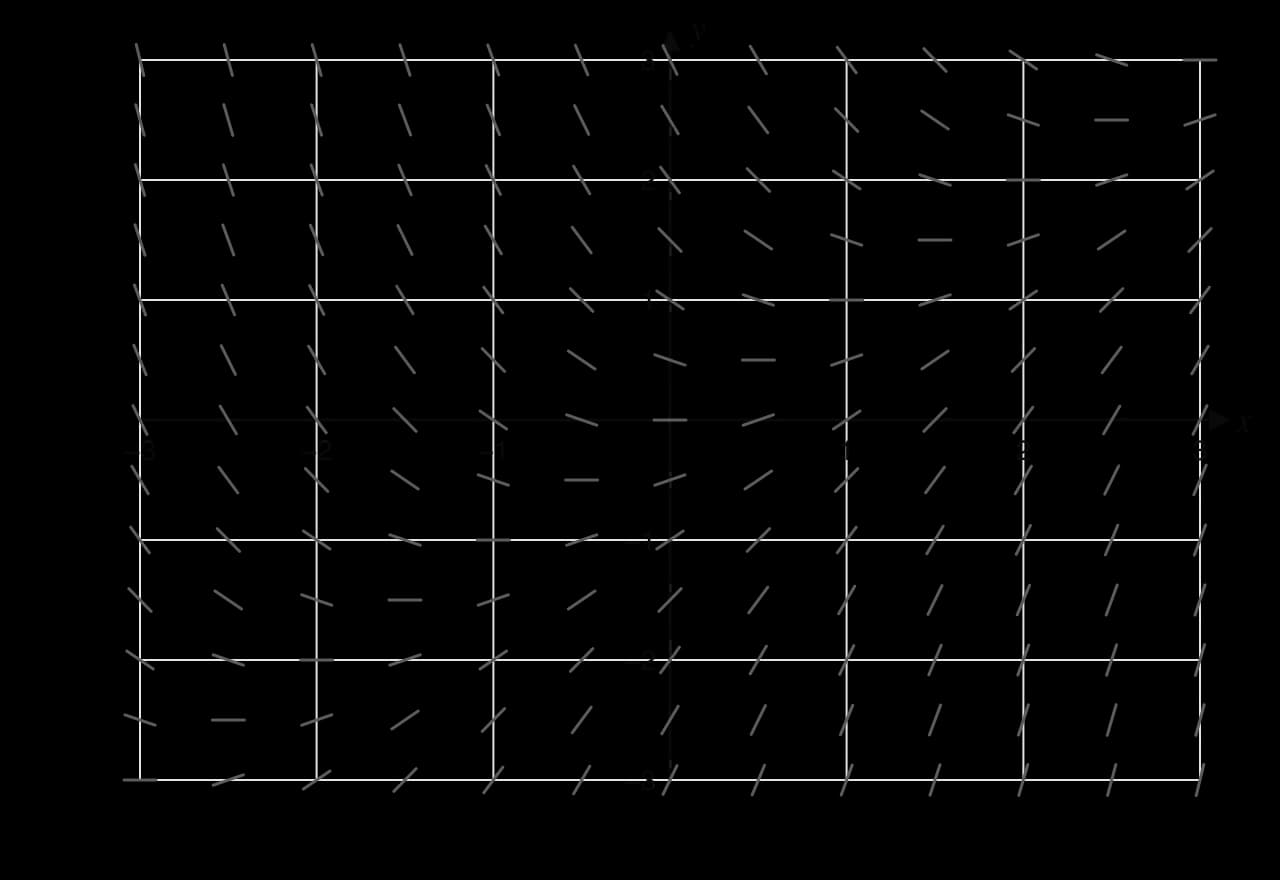
Definition

Slope field: a diagram of a first-order differential equation dydx=f(x,y)\frac{\mathrm{d}y}{\mathrm{d}x} = f(x, y)dxdy​=f(x,y) made of short line segments drawn at the points of a grid, each with gradient equal to f(x,y)f(x, y)f(x,y) at its point.

Each segment shows the direction in which a solution curve passes through that point.

Slope field for dy/dx = x − y on −3 ≤ x ≤ 3, −3 ≤ y ≤ 3 with segments every 0.5 units: flat along the line y = x, steep downward in the upper left and steep upward in the lower right.
The slope field of dy/dx = x − y: segments are horizontal along the line y = x, slope down above it and up below it, and grow steeper with distance from it.

The Khan Academy video on creating a slope field builds one point by point in exactly this way, from a table of gradients to the completed picture.
YouTube
Khan Academy, “Creating a slope field”: watch each gradient being calculated from the differential equation and drawn as a short segment at its grid point.

Worked example

For the differential equation dydx=x+y\frac{\mathrm{d}y}{\mathrm{d}x} = x + ydxdy​=x+y:

(a) Calculate the gradient of the solution curve through each of the points (1,2)(1, 2)(1,2), (−1,1)(-1, 1)(−1,1) and (−2,−1)(-2, -1)(−2,−1). [3]

(b) Write down the equation of the line on which every segment of the slope field is horizontal. [1]

(c) Describe how the segments change along the line y=1y = 1y=1 as xxx increases. [2]

Show the solution

(a) Substitute each point into x+yx + yx+y.

  • At (1,2)(1, 2)(1,2): dydx=1+2=3\frac{\mathrm{d}y}{\mathrm{d}x} = 1 + 2 = 3dxdy​=1+2=3.

  • At (−1,1)(-1, 1)(−1,1): dydx=−1+1=0\frac{\mathrm{d}y}{\mathrm{d}x} = -1 + 1 = 0dxdy​=−1+1=0, a horizontal segment.

  • At (−2,−1)(-2, -1)(−2,−1): dydx=−2+(−1)=−3\frac{\mathrm{d}y}{\mathrm{d}x} = -2 + (-1) = -3dxdy​=−2+(−1)=−3.

(b) The segments are horizontal where x+y=0x + y = 0x+y=0, that is on the line y=−xy = -xy=−x.

(c) On y=1y = 1y=1 the gradient is x+1x + 1x+1, which increases steadily with xxx: the segments slope steeply downward for large negative xxx, are horizontal at x=−1x = -1x=−1, and slope ever more steeply upward for x>−1x > -1x>−1.

Generating a slope field with technology

Drawing hundreds of segments by hand is slow, so slope fields are generated with software. In GeoGebra the command SlopeField(x - y) draws the field of dydx=x−y\frac{\mathrm{d}y}{\mathrm{d}x} = x - ydxdy​=x−y in the current window; the expression inside the brackets is the right-hand side of the equation, with xxx and yyy as the variables. Some GDCs have a differential-equation graphing mode that draws fields as well. Whatever the tool, the window should cover the region of interest, and a coarser grid (fewer segments) is often easier to read than a dense one.

Tip

To check a slope field drawn by software, substitute two or three grid points into the differential equation and compare the gradients with the segments there. A field that is horizontal where the equation says dydx=0\frac{\mathrm{d}y}{\mathrm{d}x} = 0dxdy​=0 and steep where ∣dydx∣|\frac{\mathrm{d}y}{\mathrm{d}x}|∣dxdy​∣ is large is the right one.

Solution curves

Following the field

A solution of the differential equation is a function whose graph has, at every point, exactly the gradient the equation prescribes there. On a slope field this means the graph runs along the segments: it is tangent to the field at every point it passes through. Starting at a chosen point and following the directions of nearby segments traces out that solution, much as a leaf floating on a stream follows the current.

Definition

Solution curve: the graph of a particular solution of a differential equation; on a slope field it is a smooth curve that is tangent to the segments at every point it passes through.

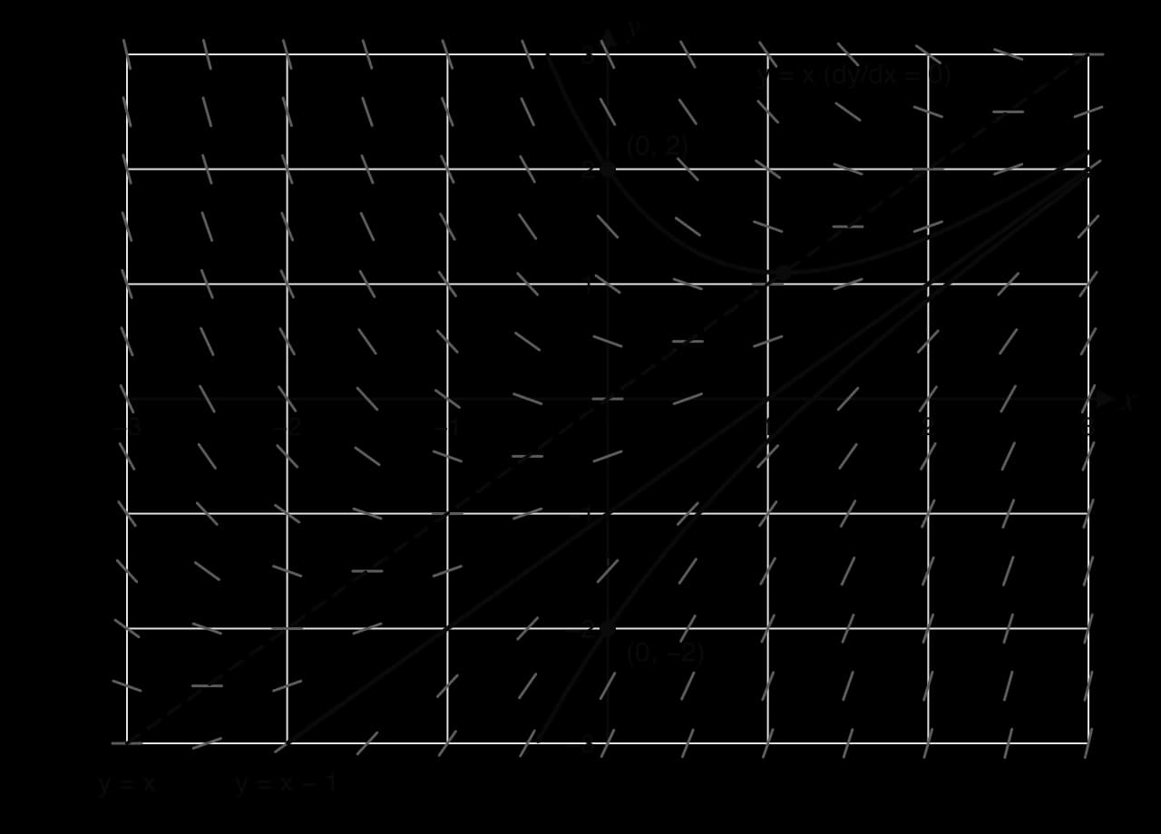
Each starting point gives a different particular solution, and together the solution curves form the general solution, the whole family. For dydx=x−y\frac{\mathrm{d}y}{\mathrm{d}x} = x - ydxdy​=x−y, the exact general solution is y=x−1+Ce−xy = x - 1 + C\mathrm{e}^{-x}y=x−1+Ce−x (it can be checked by substitution, as in subtopic 5.14). Three of its curves are drawn on the field: through (0,2)(0, 2)(0,2) with C=3C = 3C=3, through (0,−2)(0, -2)(0,−2) with C=−1C = -1C=−1, and the straight line y=x−1y = x - 1y=x−1 with C=0C = 0C=0.

Slope field for dy/dx = x − y with the dashed line y = x where dy/dx = 0, and three solution curves: through (0, 2) with a minimum at about (1.10, 1.10) on y = x, the straight line y = x − 1, and through (0, −2), all approaching y = x − 1.
Solution curves follow the segments: the curve through (0, 2) turns at its minimum on the dashed line y = x, and every solution approaches the straight-line solution y = x − 1 as x increases.

The curve through (0,2)(0, 2)(0,2) starts above the dashed line y=xy = xy=x, where the segments slope downward, so it falls. It meets the line y=xy = xy=x at about (1.10,1.10)(1.10, 1.10)(1.10,1.10), where it is momentarily horizontal, and then rises below the line. The curve through (0,−2)(0, -2)(0,−2) rises all the way. As xxx increases, the term Ce−xC\mathrm{e}^{-x}Ce−x shrinks to zero, so every solution approaches y=x−1y = x - 1y=x−1: this line is an asymptote of every other solution, which the field shows without any algebra.

The Khan Academy video on visualising solutions draws solution curves on a field in the same way, starting from different points and following the segments.
YouTube
Khan Academy, “Slope field to visualize solutions”: watch how a solution through a chosen point is sketched by following the segments of the field.

Solution curves do not cross

Two solution curves of dydx=f(x,y)\frac{\mathrm{d}y}{\mathrm{d}x} = f(x, y)dxdy​=f(x,y) cannot cross. At a crossing point both would pass through the same (x,y)(x, y)(x,y), so both would have the same gradient f(x,y)f(x, y)f(x,y), and from there the equation fixes the gradient at every next point in the same way for both. The two curves would therefore be the same curve. Solutions may come very close (as all solutions of x−yx - yx−y approach y=x−1y = x - 1y=x−1) but they never meet or cross. This holds wherever fff is a smooth function; at points where the equation is undefined, such as where a denominator is zero, the rule can fail.

Common mistake

Drawing a solution curve that crosses another solution or an asymptote, or that stops when it reaches an axis. Solution curves of a slope field never cross each other, and a curve approaching an asymptote gets ever closer without touching it. Draw the curve across the whole region shown, in both directions from the given point, unless the field itself ends it.

How to sketch a solution curve

A good sketch on a given slope field shows the right shape, passes through the right point and has the right long-term behaviour. These steps produce one.

  1. Mark the given point clearly.

  2. From the point, move a little to the right in the direction of the nearest segments, then adjust to the new segments; repeat. The curve should run between segments parallel to them, never across them.

  3. Do the same to the left of the point, so the curve covers the whole region shown.

  4. Wherever the curve crosses the curve on which dydx=0\frac{\mathrm{d}y}{\mathrm{d}x} = 0dxdy​=0, make it horizontal: that is a turning point, a local maximum or minimum of the solution.

  5. Show asymptotic behaviour: a curve approaching a line should get closer and closer without meeting it.

  6. Draw one smooth curve with no corners and no flat sections that the field does not show.

Exam tip

Examiners award one mark for a curve through the given point and further marks for the correct shape: a turning point in the right place, the right number of maxima and minima, and clear approach to an asymptote. A curve with a flat middle section where the field shows a maximum and a minimum, or one that touches or crosses an asymptote, loses the shape marks.

Isoclines and the curve where dy/dx = 0

Isoclines

Points where the field has the same gradient lie on curves called isoclines (from the Greek for "equal slope"). For dydx=f(x,y)\frac{\mathrm{d}y}{\mathrm{d}x} = f(x, y)dxdy​=f(x,y), the isocline for gradient ccc is the curve f(x,y)=cf(x, y) = cf(x,y)=c. Along it every segment is parallel, which makes isoclines a quick way to draw a field by hand: draw the curve, then add parallel segments along it.

Definition

Isocline: a curve along which every solution of a differential equation dydx=f(x,y)\frac{\mathrm{d}y}{\mathrm{d}x} = f(x, y)dxdy​=f(x,y) has the same gradient ccc; its equation is f(x,y)=cf(x, y) = cf(x,y)=c.

For dydx=x−y\frac{\mathrm{d}y}{\mathrm{d}x} = x - ydxdy​=x−y, the isocline for gradient ccc is x−y=cx - y = cx−y=c, or y=x−cy = x - cy=x−c: a family of parallel straight lines. The isocline for c=0c = 0c=0 is y=xy = xy=x, and the isocline for c=1c = 1c=1 is y=x−1y = x - 1y=x−1. That second line has gradient 1 itself, equal to the gradient of every segment on it, so the line runs along its own segments and is a solution. This is why y=x−1y = x - 1y=x−1 appeared as a straight-line solution in the field of x−yx - yx−y.

Worked example

For dydx=x2+y2\frac{\mathrm{d}y}{\mathrm{d}x} = x^2 + y^2dxdy​=x2+y2:

(a) Find the equation of the isocline on which the gradient is 4, and describe it. [2]

(b) Explain why no solution curve of this equation has a local maximum or a local minimum. [2]

Show the solution

(a) Set the right-hand side equal to 4: x2+y2=4x^2 + y^2 = 4x2+y2=4. This is the circle with centre (0,0)(0, 0)(0,0) and radius 2. Every segment on this circle has gradient 4.

(b) x2+y2≥0x^2 + y^2 \ge 0x2+y2≥0, and it equals 0 only at the single point (0,0)(0, 0)(0,0). So dydx>0\frac{\mathrm{d}y}{\mathrm{d}x} > 0dxdy​>0 everywhere else: every solution is increasing. A solution through the origin is momentarily horizontal there but increasing on both sides, so it has no maximum or minimum either (the origin is a point where the gradient is zero without a change of sign).

The nullcline holds every turning point

The most useful isocline is the one with gradient zero. At a local maximum or local minimum of a solution, the gradient is 0 (subtopic 5.6, Stationary points), so every turning point of every solution lies on the curve f(x,y)=0f(x, y) = 0f(x,y)=0. Finding this curve locates all the maxima and minima before a single solution is drawn.

Definition

Nullcline: the isocline on which dydx=0\frac{\mathrm{d}y}{\mathrm{d}x} = 0dxdy​=0, with equation f(x,y)=0f(x, y) = 0f(x,y)=0; every local maximum and local minimum of a solution curve lies on it.

For dydx=x−y\frac{\mathrm{d}y}{\mathrm{d}x} = x - ydxdy​=x−y, the nullcline is the line y=xy = xy=x.

The nullcline also splits the plane into regions where solutions rise (f>0f > 0f>0) and where they fall (f<0f < 0f<0). For x−yx - yx−y, points above y=xy = xy=x have x−y<0x - y < 0x−y<0, so solutions fall there; points below have x−y>0x - y > 0x−y>0, so solutions rise. A solution moving from the falling region into the rising region turns at a minimum, and one moving from the rising region into the falling region turns at a maximum. The curve through (0,2)(0, 2)(0,2) in the field of x−yx - yx−y passes from above y=xy = xy=x to below it, so its turning point at (ln⁡3,ln⁡3)≈(1.10,1.10)(\ln 3, \ln 3) \approx (1.10, 1.10)(ln3,ln3)≈(1.10,1.10) is a minimum.

Common mistake

Drawing a solution curve through a point where dydx=0\frac{\mathrm{d}y}{\mathrm{d}x} = 0dxdy​=0 when the question asks for the curve of points where dydx=0\frac{\mathrm{d}y}{\mathrm{d}x} = 0dxdy​=0. The nullcline is found by setting the right-hand side equal to zero and drawing the resulting equation, such as y=x2y = x^2y=x2; it is generally not a solution, and solution curves cross it horizontally.

The slope field of dydx=x2−y\frac{\mathrm{d}y}{\mathrm{d}x} = x^2 - ydxdy​=x2−y has a nullcline that is a parabola rather than a line.
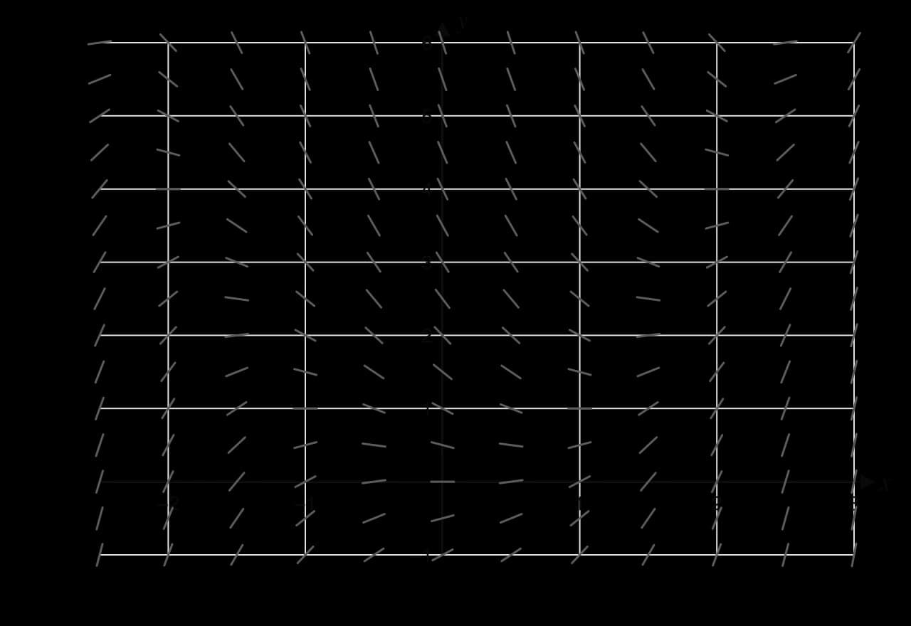
Slope field for dy/dx = x² − y on −2.5 ≤ x ≤ 3, −1 ≤ y ≤ 6, segments every 0.5 units.
The slope field of dy/dx = x² − y for −2.5 ≤ x ≤ 3: segments are horizontal along a curve shaped like a parabola.

Worked example

The slope field for the differential equation dydx=x2−y\frac{\mathrm{d}y}{\mathrm{d}x} = x^2 - ydxdy​=x2−y is shown for −2.5≤x≤3-2.5 \le x \le 3−2.5≤x≤3 and −1≤y≤6-1 \le y \le 6−1≤y≤6.

(a) Calculate the value of dydx\frac{\mathrm{d}y}{\mathrm{d}x}dxdy​ at the point (0,1)(0, 1)(0,1). [1]

(b) Write down the equation of the curve on which all the local maximum and local minimum points of the solutions lie, and sketch it on the slope field. [2]

(c) The solution through (0,1)(0, 1)(0,1) has a local maximum and a local minimum. Sketch this solution on the slope field, and state which turning point lies to the left. [3]

Show the solution

(a) dydx=02−1=−1\frac{\mathrm{d}y}{\mathrm{d}x} = 0^2 - 1 = -1dxdy​=02−1=−1.

(b) Turning points satisfy dydx=0\frac{\mathrm{d}y}{\mathrm{d}x} = 0dxdy​=0: x2−y=0x^2 - y = 0x2−y=0, so the curve is y=x2y = x^2y=x2, a parabola with its vertex at the origin.

(c) Above the parabola y>x2y > x^2y>x2, so dydx<0\frac{\mathrm{d}y}{\mathrm{d}x} < 0dxdy​<0 and solutions fall; below it they rise. The point (0,1)(0, 1)(0,1) is above the parabola, so the solution is falling there, with gradient −1-1−1.

  • Following the segments to the right, the curve falls until it meets the parabola, at about (0.77,0.59)(0.77, 0.59)(0.77,0.59), then rises below it: a local minimum.

  • Following the segments to the left from (0,1)(0, 1)(0,1), the curve gets higher, because it has negative gradient above the parabola. It meets the parabola at about (−1.68,2.82)(-1.68, 2.82)(−1.68,2.82); further left it is below the parabola, where the gradient is positive, so it is lower again. Reading from left to right, the curve rises to this point and then falls: a local maximum.

So the local maximum lies to the left of the local minimum, and both lie on y=x2y = x^2y=x2.

Slope field for dy/dx = x² − y with the dashed parabola y = x² and the solution through (0, 1), which has a local maximum near (−1.68, 2.82) and a local minimum near (0.77, 0.59), both on the parabola.
The solution through (0, 1) is horizontal exactly where it crosses the dashed parabola y = x²: a maximum on the left and a minimum on the right.

Deciding which turning points are maxima

For a nullcline that is a line or curve with a gradient of its own, the direction in which solutions cross it decides the type of turning point. A solution crosses the nullcline horizontally, so if the nullcline slopes down from left to right, every solution passes from below it to above it as xxx increases; if the nullcline slopes up, every solution passes from above it to below it. Combined with the sign of fff on each side, this identifies maxima and minima without drawing any solution.

Worked example

Solutions of dydx=sin⁡(x−y)\frac{\mathrm{d}y}{\mathrm{d}x} = \sin(x - y)dxdy​=sin(x−y) have local maxima and minima on straight lines.

(a) Show that the turning points lie on the lines y=x−nπy = x - n\piy=x−nπ, n∈Zn \in \mathbb{Z}n∈Z. [2]

(b) Determine which of these lines hold local maxima and which hold local minima. [3]

Show the solution

(a) At a turning point sin⁡(x−y)=0\sin(x - y) = 0sin(x−y)=0, so x−y=nπx - y = n\pix−y=nπ for an integer nnn, that is y=x−nπy = x - n\piy=x−nπ.

(b) Each line has gradient 111, and a solution crosses it horizontally (gradient 0), so as xxx increases the line rises past the solution: every solution passes from above the line to below it.

  • On the line y=xy = xy=x (x−y=0x - y = 0x−y=0): just above it, x−yx - yx−y is a little less than 0, so sin⁡(x−y)<0\sin(x - y) < 0sin(x−y)<0 and the solution falls; just below, x−yx - yx−y is a little more than 0, so sin⁡(x−y)>0\sin(x - y) > 0sin(x−y)>0 and it rises. Falling then rising: local minima lie on y=xy = xy=x.

  • On the line y=x−πy = x - \piy=x−π (x−y=πx - y = \pix−y=π): just above, x−yx - yx−y is a little less than π\piπ, so sin⁡(x−y)>0\sin(x - y) > 0sin(x−y)>0 (rising); just below, x−yx - yx−y is a little more than π\piπ, so sin⁡(x−y)<0\sin(x - y) < 0sin(x−y)<0 (falling). Rising then falling: local maxima lie on y=x−πy = x - \piy=x−π.

The pattern repeats every 2π2\pi2π: minima on y=x−2kπy = x - 2k\piy=x−2kπ and maxima on y=x−π−2kπy = x - \pi - 2k\piy=x−π−2kπ, k∈Zk \in \mathbb{Z}k∈Z (radians throughout).

Linking question: How is a slope field related to Euler's method? Euler's method (subtopic 5.16) starts at a point, moves along the segment there for a short step of fixed horizontal length, and repeats from the new point. It is a numerical version of sketching a solution on a slope field, with straight steps in place of a smooth curve, so its error grows where the field changes direction quickly.

Patterns in slope fields

Equations that depend on x only

When the right-hand side contains only xxx, as in dydx=cos⁡x\frac{\mathrm{d}y}{\mathrm{d}x} = \cos xdxdy​=cosx or dydx=2x\frac{\mathrm{d}y}{\mathrm{d}x} = 2xdxdy​=2x, the gradient is the same at every point of a vertical line. The field repeats exactly as it moves up or down, so every solution curve is a vertical translation of every other. This matches the general solution y=∫f(x) dx+cy = \int f(x)\,\mathrm{d}x + cy=∫f(x)dx+c of subtopic 5.14, where changing ccc shifts the curve vertically.

Autonomous equations

When the right-hand side contains only the unknown, as in dPdt=0.5P(1−P10)\frac{\mathrm{d}P}{\mathrm{d}t} = 0.5P\left(1 - \frac{P}{10}\right)dtdP​=0.5P(1−10P​), the rate of change does not depend on the time. The gradient is then the same along every horizontal line, so each row of the field is identical and solutions are horizontal translations of one another: starting the same population later gives the same curve shifted to the right.

Definition

Autonomous differential equation: a first-order differential equation dydx=f(y)\frac{\mathrm{d}y}{\mathrm{d}x} = f(y)dxdy​=f(y) whose right-hand side depends only on the unknown yyy and not on the independent variable.

Newton's law of cooling, dTdt=−k(T−20)\frac{\mathrm{d}T}{\mathrm{d}t} = -k(T - 20)dtdT​=−k(T−20), and the logistic equation are autonomous.

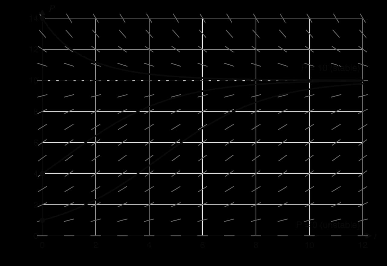
The values of yyy where f(y)=0f(y) = 0f(y)=0 give horizontal segments all the way across the field, so the horizontal lines at those heights are themselves solutions, the equilibrium solutions. The field of the logistic equation dPdt=0.5P(1−P10)\frac{\mathrm{d}P}{\mathrm{d}t} = 0.5P\left(1 - \frac{P}{10}\right)dtdP​=0.5P(1−10P​) has two: P=0P = 0P=0 and P=10P = 10P=10.

Slope field for dP/dt = 0.5P(1 − P/10), 0 ≤ t ≤ 12, 0 ≤ P ≤ 14: segments repeat along horizontal lines; flat at P = 0 and at the dashed line P = 10. Solutions from P = 1, 4 and 14 all approach P = 10.
In the field of an autonomous equation every row of segments is identical; solutions starting above or below P = 10 all approach it, while solutions move away from P = 0.

Between 0 and 10 the segments slope upward, steepest at P=5P = 5P=5 where dPdt=0.5×5×0.5=1.25\frac{\mathrm{d}P}{\mathrm{d}t} = 0.5 \times 5 \times 0.5 = 1.25dtdP​=0.5×5×0.5=1.25, so populations grow with an S-shaped curve towards 10, the carrying capacity. Above 10 the segments slope downward, so a population that starts above the carrying capacity falls towards it. Solutions on both sides approach P=10P = 10P=10, so it is a stable equilibrium; solutions near P=0P = 0P=0 move away from it, so P=0P = 0P=0 is unstable. The same reasoning applied to the cooling field dTdt=−0.1(T−20)\frac{\mathrm{d}T}{\mathrm{d}t} = -0.1(T - 20)dtdT​=−0.1(T−20) shows a single stable equilibrium at room temperature, T=20T = 20T=20.

Common mistake

Drawing a solution that reaches an equilibrium line, such as P=10P = 10P=10, at a corner and then runs along it. The horizontal line is itself a solution, so no other solution can meet it; a solution starting at P=4P = 4P=4 bends over smoothly and gets ever closer to P=10P = 10P=10 without arriving. In the logistic field the curve from P=4P = 4P=4 is still slightly below 10 at the right-hand edge.

Stability can be read from the signs of the rate on either side of each equilibrium, without drawing the field: if the rate is positive just below and negative just above, nearby solutions move towards the equilibrium from both sides.

Worked example

The population NNN (thousands) of a species of fish in a lake is modelled by dNdt=0.2N(6−N)\frac{\mathrm{d}N}{\mathrm{d}t} = 0.2N(6 - N)dtdN​=0.2N(6−N), where ttt is in years. (Hypothetical model.)

(a) Explain why the slope field of this equation looks the same along every horizontal line. [1]

(b) Find the equilibrium solutions, and state whether each is stable or unstable. [4]

(c) Describe the solution curves that start at N=1N = 1N=1 and at N=8N = 8N=8. [2]

Show the solution

(a) The right-hand side depends only on NNN, not on ttt: the equation is autonomous, so the gradient at (t,N)(t, N)(t,N) is the same for every ttt.

(b) Set 0.2N(6−N)=00.2N(6 - N) = 00.2N(6−N)=0: N=0N = 0N=0 or N=6N = 6N=6.

  • For 0<N<60 < N < 60<N<6: dNdt>0\frac{\mathrm{d}N}{\mathrm{d}t} > 0dtdN​>0, so solutions rise towards 6. For N>6N > 6N>6: dNdt<0\frac{\mathrm{d}N}{\mathrm{d}t} < 0dtdN​<0, so solutions fall towards 6. Solutions on both sides approach 6: N=6N = 6N=6 is stable.

  • Just above 0, solutions rise away from 0: N=0N = 0N=0 is unstable.

(c) From N=1N = 1N=1: the curve rises in an S shape, steepest at N=3N = 3N=3 (where 0.2N(6−N)0.2N(6 - N)0.2N(6−N) is greatest, 1.81.81.8 thousand fish per year), and approaches N=6N = 6N=6 from below without reaching it. From N=8N = 8N=8: the curve falls, steeply at first and then more gently, approaching N=6N = 6N=6 from above. Neither curve crosses N=6N = 6N=6.

Reading a slope field

Most features of a slope field can be predicted from its equation, and most features of an equation can be recognised in its field. The table collects the patterns that identify a field.

Feature of the equation dydx=f(x,y)\frac{\mathrm{d}y}{\mathrm{d}x} = f(x, y)dxdy​=f(x,y)

What it looks like in the slope field

fff depends on xxx only

segments identical along each vertical line

fff depends on yyy only (autonomous)

segments identical along each horizontal line

f(x,y)=0f(x, y) = 0f(x,y)=0 on a curve

horizontal segments along that curve (the nullcline)

fff undefined on a line, e.g. xy\frac{x}{y}yx​ at y=0y = 0y=0

vertical segments along that line

f(−x,y)=−f(x,y)f(-x, y) = -f(x, y)f(−x,y)=−f(x,y)

field symmetric in the yyy-axis (mirror image)

fff has the same sign everywhere

all segments slope the same way; solutions have no turning points

f(y)=0f(y) = 0f(y)=0 at y=cy = cy=c

the horizontal line y=cy = cy=c is a solution (an equilibrium)

Worked example

Four differential equations are given.

A: dydx=y\frac{\mathrm{d}y}{\mathrm{d}x} = ydxdy​=y B: dydx=x\frac{\mathrm{d}y}{\mathrm{d}x} = xdxdy​=x C: dydx=−xy\frac{\mathrm{d}y}{\mathrm{d}x} = -\frac{x}{y}dxdy​=−yx​ D: dydx=x+y\frac{\mathrm{d}y}{\mathrm{d}x} = x + ydxdy​=x+y

State which equation has each slope field described, giving a reason. [4]

(i) Segments are horizontal along the yyy-axis and vertical along the xxx-axis.

(ii) Segments are identical along every horizontal line and horizontal along the xxx-axis.

(iii) Segments are horizontal along the line y=−xy = -xy=−x.

(iv) Segments are identical along every vertical line and horizontal along the yyy-axis.

Show the solution

(i) C: −xy=0-\frac{x}{y} = 0−yx​=0 when x=0x = 0x=0 (the yyy-axis), and it is undefined, giving vertical segments, when y=0y = 0y=0 (the xxx-axis). (Its solution curves are circles centred at the origin.)

(ii) A: the gradient depends only on yyy (autonomous), and y=0y = 0y=0 on the xxx-axis.

(iii) D: x+y=0x + y = 0x+y=0 on the line y=−xy = -xy=−x.

(iv) B: the gradient depends only on xxx, and x=0x = 0x=0 on the yyy-axis. (Its solutions are the parabolas y=x22+cy = \frac{x^2}{2} + cy=2x2​+c.)

Slope fields in the world

Wind maps such as earth.nullschool.net show the wind across the globe as short moving lines on a grid, drawn from the Global Forecast System model of the United States National Oceanic and Atmospheric Administration (NOAA). Each line shows the wind's direction at that place, so the map is a direction field in two dimensions, and a balloon drifting with the wind follows a path tangent to the lines, as a solution curve follows its field. The analogy holds only while the wind pattern stays the same; real winds change from hour to hour, so a real balloon follows a changing field.

Key concept: Representation. A slope field represents a differential equation as a picture, showing the shape of every solution at once without solving anything. Each representation of the same equation (a formula, a field, a table of Euler steps) makes different features easy to see. The field shows equilibria and long-term behaviour at a glance, and a formula gives exact values.

Tip

Improve your notes: For each of dydx=x−y\frac{\mathrm{d}y}{\mathrm{d}x} = x - ydxdy​=x−y, dydx=x2−y\frac{\mathrm{d}y}{\mathrm{d}x} = x^2 - ydxdy​=x2−y and dPdt=0.5P(1−P10)\frac{\mathrm{d}P}{\mathrm{d}t} = 0.5P\left(1 - \frac{P}{10}\right)dtdP​=0.5P(1−10P​), generate the slope field with GeoGebra's SlopeField command, sketch it, add the nullcline in a different style and draw three solution curves. Next to each, write which turning points are maxima and which are minima, and the long-term behaviour.

Theory of knowledge: A slope field is drawn with a grid spacing, a window and a segment length chosen by its maker, and these choices decide which features a reader sees: too coarse a grid can hide a turning point, and too small a window can hide an asymptote. In what ways do the choices of the person drawing a diagram shape the knowledge a reader takes from it?

Exam focus

Slope fields are examined on HL Paper 1 in short questions of 2 to 7 marks, with the field printed on the paper. The usual parts are: calculate dydx\frac{\mathrm{d}y}{\mathrm{d}x}dxdy​ at a given point (substitution); write down or find the equation of the curve on which the maxima and minima of the solutions lie (set the right-hand side to zero and rearrange); sketch that curve on the field; sketch the solution curve through one or two given points. Markschemes award marks for the correct gradient, the curve through the given point, turning points on the nullcline and clear asymptotic behaviour.

The examiners' reports describe these questions as often left blank, and the commonest error as drawing a solution through the point where dydx=0\frac{\mathrm{d}y}{\mathrm{d}x} = 0dxdy​=0 instead of the curve of all such points. Sketches also lose marks for flat sections, missing turning points and curves that touch, cross or stop at an asymptote.

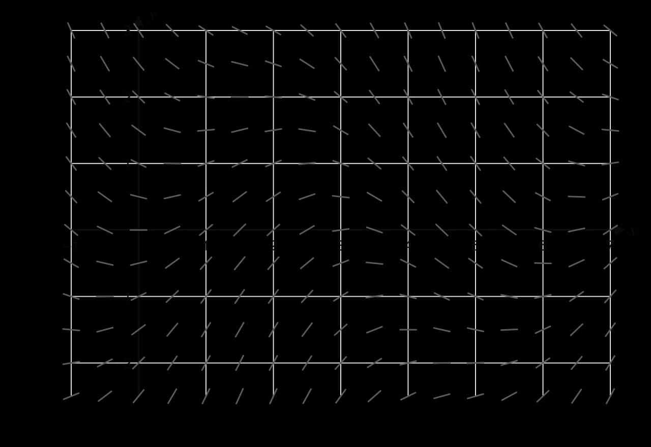
The slope field of dydx=sin⁡x−y2\frac{\mathrm{d}y}{\mathrm{d}x} = \sin x - \frac{y}{2}dxdy​=sinx−2y​, drawn for −1≤x≤7-1 \le x \le 7−1≤x≤7 and −2.5≤y≤3-2.5 \le y \le 3−2.5≤y≤3, is used in the following question.

Slope field for dy/dx = sin x − y/2 on −1 ≤ x ≤ 7, −2.5 ≤ y ≤ 3, segments every 0.5 units.
The slope field of dy/dx = sin x − y/2 for −1 ≤ x ≤ 7 and −2.5 ≤ y ≤ 3 (x in radians).

Exam tip

The slope field for the differential equation dydx=sin⁡x−y2\frac{\mathrm{d}y}{\mathrm{d}x} = \sin x - \frac{y}{2}dxdy​=sinx−2y​, for −1≤x≤7-1 \le x \le 7−1≤x≤7, is shown.

(a) Calculate the value of dydx\frac{\mathrm{d}y}{\mathrm{d}x}dxdy​ at the point (0,2)(0, 2)(0,2). [1]

(b) Write down the equation of the curve on which all the local maximum and local minimum points of the solution curves lie. [1]

(c) Sketch this curve on the slope field. [2]

(d) Sketch the solution curve that passes through (0,2)(0, 2)(0,2). [3]

(e) The first local minimum of the solution through (0,2)(0, 2)(0,2) occurs at x=0.928x = 0.928x=0.928. Find the yyy-coordinate of this point. [2]

Show the markscheme

(a) dydx=sin⁡0−22=−1\frac{\mathrm{d}y}{\mathrm{d}x} = \sin 0 - \frac{2}{2} = -1dxdy​=sin0−22​=−1 A1

(b) sin⁡x−y2=0⇒y=2sin⁡x\sin x - \frac{y}{2} = 0 \Rightarrow y = 2\sin xsinx−2y​=0⇒y=2sinx A1

(c) sine curve through the origin with amplitude 2 A1, maximum near (1.57,2)(1.57, 2)(1.57,2), minimum near (4.71,−2)(4.71, -2)(4.71,−2), crossing the xxx-axis near 3.14 and 6.28 A1

(d) curve through (0,2)(0, 2)(0,2) with negative gradient there A1

local minimum then local maximum on y=2sin⁡xy = 2\sin xy=2sinx (near x=0.93x = 0.93x=0.93 and x=2.10x = 2.10x=2.10) A1

decreasing to a local minimum on y=2sin⁡xy = 2\sin xy=2sinx near (5.9,−0.74)(5.9, -0.74)(5.9,−0.74), then increasing A1

Slope field for dy/dx = sin x − y/2 with the dashed curve y = 2 sin x and the solution through (0, 2): a local minimum near (0.93, 1.60), a maximum near (2.10, 1.73) and a minimum near (5.90, −0.74), all on y = 2 sin x.
The solution through (0, 2) is horizontal exactly where it meets the dashed curve y = 2 sin x: minimum, maximum, then minimum.

(e) the minimum lies on y=2sin⁡xy = 2\sin xy=2sinx (M1)

y=2sin⁡0.928=1.60y = 2\sin 0.928 = 1.60y=2sin0.928=1.60 A1

Total [9]

Part (e) needs no solving of the differential equation: once the xxx-coordinate of a turning point is known, the nullcline gives its yyy-coordinate. Questions of this kind reward understanding of the link between dydx=0\frac{\mathrm{d}y}{\mathrm{d}x} = 0dxdy​=0 and turning points more than calculation.

Exam tip

Draw solution curves in pencil first, lightly, testing them against the segments every few millimetres, then go over the final curve firmly. Mark each turning point on the nullcline you have drawn, and extend every curve to the edges of the field so that its long-term behaviour, such as approaching an asymptote, can be seen.

Practice questions

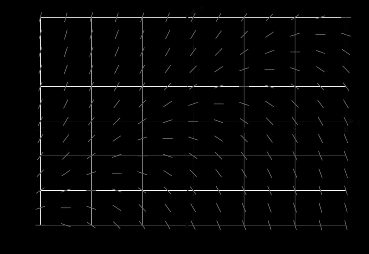
The slope field of dydx=y−x\frac{\mathrm{d}y}{\mathrm{d}x} = y - xdxdy​=y−x for −3≤x≤3-3 \le x \le 3−3≤x≤3 and −3≤y≤3-3 \le y \le 3−3≤y≤3 is used in questions 1 to 4.

Slope field for dy/dx = y − x on −3 ≤ x ≤ 3, −3 ≤ y ≤ 3 with segments every 0.5 units.
The slope field of dy/dx = y − x for practice questions 1 to 4.
  1. Calculate the gradient of the solution curve through (1,3)(1, 3)(1,3) and through (2,−2)(2, -2)(2,−2). [2]

  2. Write down the equation of the curve on which every segment is horizontal. [1]

  3. Show that the line y=x+1y = x + 1y=x+1 is a solution curve of the differential equation. [2]

  4. (a) Sketch the solution curve through (0,0)(0, 0)(0,0). (b) Explain why it has a local maximum at the origin. (c) Describe the long-term behaviour of the solutions through (0,2)(0, 2)(0,2) and (0,0)(0, 0)(0,0) as xxx increases. [6]

  5. Find the equation of the isocline on which the gradient is 2 for dydx=xy\frac{\mathrm{d}y}{\mathrm{d}x} = xydxdy​=xy, and describe the slope field on the coordinate axes. [3]

  6. For dydx=x−y2\frac{\mathrm{d}y}{\mathrm{d}x} = x - y^2dxdy​=x−y2, write down the equation of the curve on which all turning points of solutions lie, and describe its shape. [2]

  7. For the autonomous equation dydt=y(3−y)(y+2)\frac{\mathrm{d}y}{\mathrm{d}t} = y(3 - y)(y + 2)dtdy​=y(3−y)(y+2), find the equilibrium solutions and determine whether each is stable or unstable. [5]

  8. Explain why every solution curve of dydx=3x2−4\frac{\mathrm{d}y}{\mathrm{d}x} = 3x^2 - 4dxdy​=3x2−4 is a vertical translation of the curve through the origin, and write down the equation of that curve. [3]

  9. State, with a reason, which of dydx=yx\frac{\mathrm{d}y}{\mathrm{d}x} = \frac{y}{x}dxdy​=xy​ and dydx=−yx\frac{\mathrm{d}y}{\mathrm{d}x} = -\frac{y}{x}dxdy​=−xy​ has a slope field in which the segments all point along lines through the origin. [2]

Answers
  1. At (1,3)(1, 3)(1,3): 3−1=23 - 1 = 23−1=2. At (2,−2)(2, -2)(2,−2): −2−2=−4-2 - 2 = -4−2−2=−4.

  2. y−x=0y - x = 0y−x=0, so y=xy = xy=x.

  3. On y=x+1y = x + 1y=x+1, dydx=1\frac{\mathrm{d}y}{\mathrm{d}x} = 1dxdy​=1 (the line's gradient) and y−x=(x+1)−x=1y - x = (x + 1) - x = 1y−x=(x+1)−x=1. The two agree at every point, so the line is a solution.

  4. (a) A curve through the origin, horizontal there, falling on both sides (the exact solution is y=x+1−exy = x + 1 - \mathrm{e}^{x}y=x+1−ex). (b) At (0,0)(0, 0)(0,0), y−x=0y - x = 0y−x=0 so the gradient is 0; for x<0x < 0x<0 the curve lies above y=xy = xy=x (gradient positive, rising) and for x>0x > 0x>0 below it (gradient negative, falling), so the turning point is a maximum. (c) The solution through (0,2)(0, 2)(0,2) lies above y=x+1y = x + 1y=x+1 and rises ever more steeply; the solution through (0,0)(0, 0)(0,0) lies below y=x+1y = x + 1y=x+1 and falls ever more steeply. Solutions move away from y=x+1y = x + 1y=x+1 as xxx increases.

  5. xy=2xy = 2xy=2, the hyperbola y=2xy = \frac{2}{x}y=x2​. On both axes xy=0xy = 0xy=0, so every segment on the xxx-axis and on the yyy-axis is horizontal.

  6. x−y2=0x - y^2 = 0x−y2=0, so x=y2x = y^2x=y2: a parabola opening to the right with vertex at the origin.

  7. y=−2y = -2y=−2, y=0y = 0y=0 and y=3y = 3y=3. Sign of y(3−y)(y+2)y(3 - y)(y + 2)y(3−y)(y+2): for y<−2y < -2y<−2, two factors are negative (yyy and y+2y + 2y+2), so the product is positive; for −2<y<0-2 < y < 0−2<y<0, negative; for 0<y<30 < y < 30<y<3, positive; for y>3y > 3y>3, negative. So solutions rise towards −2-2−2 from below and fall towards it from above: y=−2y = -2y=−2 stable; they move away from y=0y = 0y=0 on both sides: unstable; they approach y=3y = 3y=3 from both sides: stable.

  8. The right-hand side depends on xxx only, so the gradient is the same at every point of a vertical line and y=x3−4x+cy = x^3 - 4x + cy=x3−4x+c; changing ccc shifts the curve vertically. Through the origin, c=0c = 0c=0: y=x3−4xy = x^3 - 4xy=x3−4x.

  9. dydx=yx\frac{\mathrm{d}y}{\mathrm{d}x} = \frac{y}{x}dxdy​=xy​: at (x,y)(x, y)(x,y) the segment has gradient yx\frac{y}{x}xy​, the gradient of the line from the origin to that point, so every segment points along a line through the origin (its solutions are the lines y=kxy = kxy=kx).

Summary

  • A slope field draws a short segment with gradient f(x,y)f(x, y)f(x,y) at each grid point for dydx=f(x,y)\frac{\mathrm{d}y}{\mathrm{d}x} = f(x, y)dxdy​=f(x,y); the gradient at a point comes from substituting into the equation.

  • Software draws fields, for example GeoGebra's SlopeField(f(x, y)); checking two or three gradients confirms the field is right.

  • A solution curve is tangent to the segments everywhere; sketch it smoothly through the given point, in both directions, showing turning points and asymptotes.

  • Solution curves never cross, because at a shared point they would have the same gradient and so be the same curve.

  • An isocline f(x,y)=cf(x, y) = cf(x,y)=c joins points with equal gradient; an isocline that is a line with gradient ccc is itself a solution.

  • The nullcline f(x,y)=0f(x, y) = 0f(x,y)=0 holds every local maximum and minimum of every solution; it is not itself a solution in general.

  • A solution passing from a region where f>0f > 0f>0 to one where f<0f < 0f<0 has a maximum on the nullcline; from f<0f < 0f<0 to f>0f > 0f>0, a minimum.

  • Fields of dydx=f(x)\frac{\mathrm{d}y}{\mathrm{d}x} = f(x)dxdy​=f(x) repeat vertically (solutions are vertical translations); fields of autonomous equations dydx=f(y)\frac{\mathrm{d}y}{\mathrm{d}x} = f(y)dxdy​=f(y) repeat horizontally, with equilibrium solutions where f(y)=0f(y) = 0f(y)=0, stable when nearby solutions approach them.

Self-check

  • To do:

    I can calculate dydx\frac{\mathrm{d}y}{\mathrm{d}x}dxdy​ at any point by substituting into the differential equation.

  • To do:

    I can explain how a slope field is built from a grid of gradients.

  • To do:

    I can generate a slope field with technology and check it against the equation.

  • To do:

    I can sketch a smooth solution curve through a given point in both directions.

  • To do:

    I can explain why two solution curves cannot cross.

  • To do:

    I can find the equation of an isocline for a given gradient.

  • To do:

    I can find and sketch the curve on which dydx=0\frac{\mathrm{d}y}{\mathrm{d}x} = 0dxdy​=0, and avoid drawing a solution through a single point instead.

  • To do:

    I can decide whether a turning point on the nullcline is a maximum or a minimum from the signs of dydx\frac{\mathrm{d}y}{\mathrm{d}x}dxdy​ on each side.

  • To do:

    I can use the nullcline to find a coordinate of a turning point.

  • To do:

    I can recognise an autonomous equation from its field and find its equilibrium solutions.

  • To do:

    I can decide whether an equilibrium is stable or unstable from the field or the sign of the rate.

  • To do:

    I can show approach to an asymptote clearly without touching or crossing it.

  • To do:

    I can match a differential equation to its slope field from its features.

Questions on 5.15

18 exam-style questions on this subtopic, written in the style of the IB papers. The first has its markscheme open. Counted on 20 October 2026

Question 1 · AI-016597 marks

The following diagram shows the slope field for the differential equation
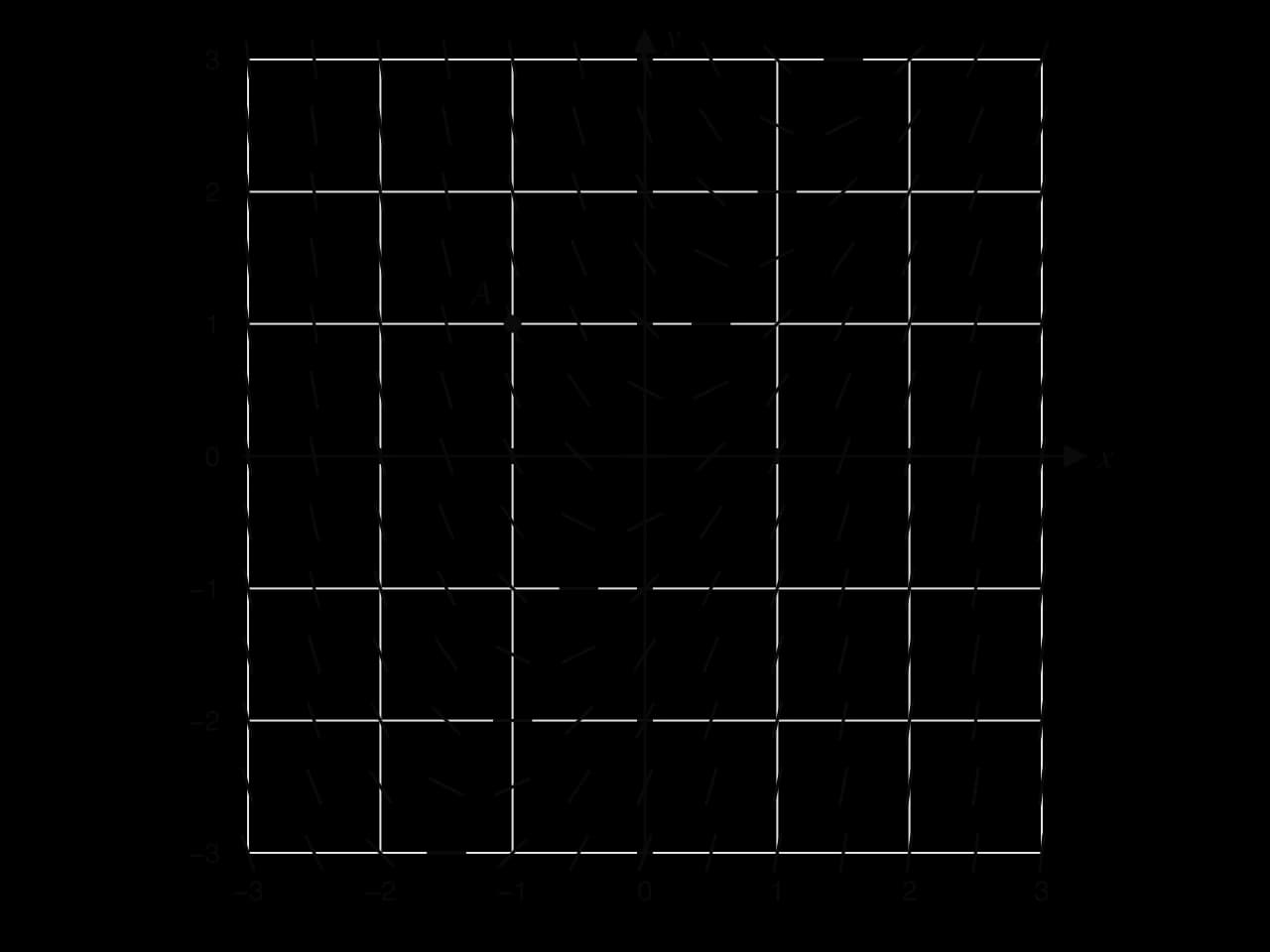
dydx=2x−y.\frac{\mathrm{d}y}{\mathrm{d}x} = 2x - y.dxdy​=2x−y.
Slope field for dy/dx = 2x − y on the grid −3 ≤ x ≤ 3, −3 ≤ y ≤ 3, with short line segments every 0.5 units. The point A(−1, 1) is marked.

The point A(−1,1)A(-1, 1)A(−1,1) lies on one of the solution curves.

  1. (a)

    Find the equation of the tangent to this solution curve at AAA. Give your answer in the form ax+by+d=0ax + by + d = 0ax+by+d=0, where a,b,d∈Za, b, d \in \mathbb{Z}a,b,d∈Z.

    [2]2 marks

    Markscheme (a)

    gradient at AAA =2(−1)−1=−3= 2(-1) - 1 = -3=2(−1)−1=−3 (A1)

    y−1=−3(x+1)y - 1 = -3(x + 1)y−1=−3(x+1), so 3x+y+2=03x + y + 2 = 03x+y+2=0 A1

    Note: Accept any integer multiple, e.g. −3x−y−2=0-3x - y - 2 = 0−3x−y−2=0.

    [2 marks]

  2. (b)

    On the diagram, sketch the solution curve that passes through AAA.

    [2]2 marks

    Markscheme (b)

    curve through AAA with a negative gradient at AAA, decreasing to a minimum close to (−0.1,−0.2)(-0.1, -0.2)(−0.1,−0.2) A1

    then increasing for larger xxx, following the field and approaching (but not crossing) the line y=2x−2y = 2x - 2y=2x−2 A1

    Note: The curve must not cut across the segments. The minimum must lie on the line y=2xy = 2xy=2x.

    [2 marks]

  3. (c)

    Write down the equation of the line on which every solution curve has a gradient of zero.

    [1]1 mark

    Markscheme (c)

    y=2xy = 2xy=2x A1

    [1 mark]

  4. (d)

    Show that y=2x−2y = 2x - 2y=2x−2 is a solution of the differential equation.

    [2]2 marks

    Markscheme (d)

    dydx=2\dfrac{\mathrm{d}y}{\mathrm{d}x} = 2dxdy​=2 M1

    2x−y=2x−(2x−2)=22x - y = 2x - (2x - 2) = 22x−y=2x−(2x−2)=2 A1

    so y=2x−2y = 2x - 2y=2x−2 satisfies the differential equation AG

    [2 marks]

Question 2 · AI-016606 marks

The following diagram shows the slope field for the differential equation
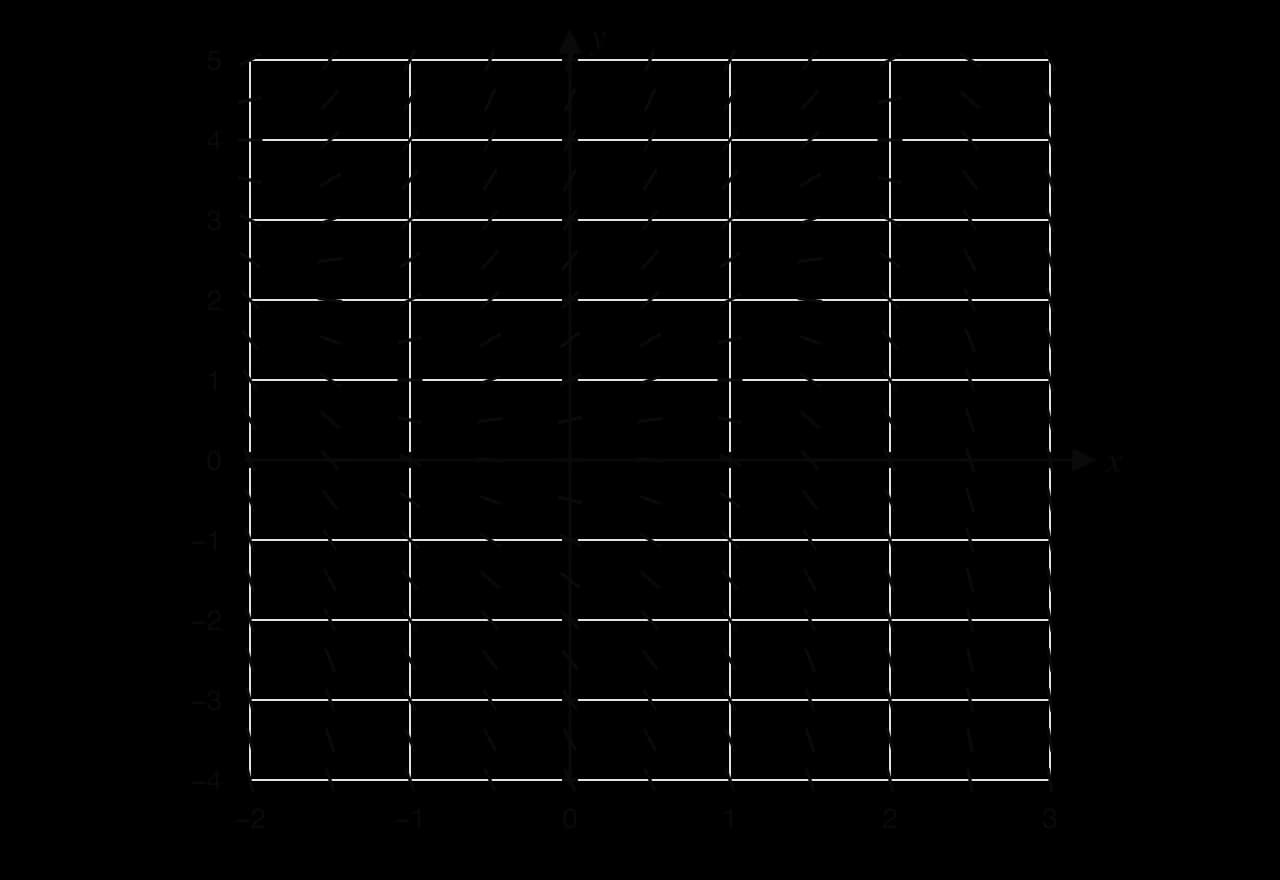
dydx=y−x2.\frac{\mathrm{d}y}{\mathrm{d}x} = y - x^2.dxdy​=y−x2.
Slope field for dy/dx = y − x² for −2 ≤ x ≤ 3 and −4 ≤ y ≤ 5, with line segments every 0.5 units.
  1. (a)(i)

    Write down the equation of the curve on which every local maximum and local minimum of the solution curves lies.

    [1]1 mark

  2. (a)(ii)

    Sketch this curve on the diagram.

    [1]1 mark

  3. (b)

    On the diagram, sketch the solution curve that passes through the point (0,1)(0, 1)(0,1).

    [2]2 marks

  4. (c)

    The solution curve through (0,1)(0, 1)(0,1) has a turning point at which x<0x < 0x<0. Determine whether this turning point is a local maximum or a local minimum. Justify your answer.

    [2]2 marks

Answer it, then compare with the markscheme.Check this one with a free account
Question 3 · AI-016615 marks

The following diagrams show the slope fields of three differential equations.
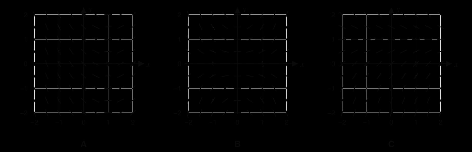
Three slope fields A, B and C, each for −2 ≤ x ≤ 2 and −2 ≤ y ≤ 2 with segments every 0.5 units. A: segments parallel within each vertical column, horizontal along x = 1. B: segments horizontal along both axes. C: segments parallel within each horizontal row, horizontal along y = 1.

The three differential equations are

(I) dydx=1−y(II) dydx=x−1(III) dydx=xy\text{(I) } \frac{\mathrm{d}y}{\mathrm{d}x} = 1 - y \qquad \text{(II) } \frac{\mathrm{d}y}{\mathrm{d}x} = x - 1 \qquad \text{(III) } \frac{\mathrm{d}y}{\mathrm{d}x} = xy(I) dxdy​=1−y(II) dxdy​=x−1(III) dxdy​=xy
  1. (a)

    Match each differential equation to its slope field. Give a reason for each choice.

    [3]3 marks

  2. (b)

    For differential equation (I), write down the equilibrium solution and describe the long-term behaviour of every other solution.

    [2]2 marks

Answer it, then compare with the markscheme.Check this one with a free account

From the formula booklet

The entries of the mathematics: applications and interpretation formula booklet that 5.15 uses. Each opens in the explained booklet.

  • Euler’s method stepTopic 5: Calculus › HL only › AHL 5.16 Euler’s methodyn+1=yn+h×f(xn,yn)y_{n+1} = y_n + h \times f(x_n, y_n)yn+1​=yn​+h×f(xn​,yn​)
  • Euler’s method x-stepTopic 5: Calculus › HL only › AHL 5.16 Euler’s methodxn+1=xn+hx_{n+1} = x_n + hxn+1​=xn​+h

On this page

  • Key terms
  • Notes
  • Questions
  • Formula booklet

Published for 5.15

Exam-style questions
18
Notes pages
1
Key terms
5
Counted on 20 October 2026Open it in Augment

More of IB Maths AI

  • 5.14 Setting up differential equationsBefore this in the Maths AI syllabus.
  • 5.16 Euler’s methodAfter this in the Maths AI syllabus.
  • 5 CalculusThe whole topic, with all 18 of its subtopics.
  • IB Maths AIThe Maths AI syllabus, assessment and what Augment has for it.

Carry on with 5.15 in Augment

With a free account, Augment remembers where you stopped and what you have practiced.

Start freeOpen 5.15 in Augment