5.1 Limits and the derivative

Introduction

Calculus is the mathematics of change. Many quantities change at a rate that is itself changing: a car speeds up and slows down, the cost of making one more item depends on how many are already being made, and the concentration of carbon dioxide in the atmosphere rises faster now than it did fifty years ago. Algebra and the gradient of a straight line can describe a constant rate of change. Describing a rate that varies needs a new idea, the derivative, which gives the rate of change at a single instant.

The derivative rests on the idea of a limit: the value a quantity gets closer and closer to as something else approaches a chosen value. A car's speedometer shows a limit at work. It cannot measure speed over an interval of zero length, so it measures distance over a very short time and divides; the shorter the time, the closer the reading is to the speed at that instant.

The idea of a limit

A limit describes where the values of a function are heading, rather than where they are. Sometimes a function cannot be evaluated at a point at all, because the formula breaks down there, yet its values close to that point settle towards one number. That number is the limit.

The arrow $\to$ is read "tends to" or "approaches". The statement $x \to a$ means that $x$ takes values nearer and nearer to $a$, from both sides, without needing to equal $a$. The value of the function at $a$ itself plays no part in the limit: the function might be undefined there, or defined with a different value.

Estimating a limit from a table of values

The function $g(x) = \frac{2^x - 1}{x}$ has no value at $x = 0$, because substituting 0 gives $\frac{0}{0}$, which is undefined. A table of values for $x$ close to 0, on both sides, shows what happens near that point.

From the left the values rise towards about 0.693, and from the right they fall towards the same number. Both sides approach the same value, so the limit exists and

The table cannot prove the limit or give it exactly; it gives evidence. The evidence is strong when the values from both sides agree to more and more decimal places as $x$ moves closer to 0. In this case the exact limit is $\ln 2 = 0.693147\ldots$, but recognising the exact value is not part of the method: an estimate to 3 significant figures, supported by a table, is the aim.

Estimating a limit from a graph

A graph shows the same behaviour as a table. The graph of $g(x) = \frac{2^x - 1}{x}$ is a smooth curve with a single missing point, drawn as an open circle, at $x = 0$. Following the curve towards $x = 0$ from either side leads to the height of the missing point, which is the limit.

On a GDC the missing point is usually invisible, because the screen shows pixels and the gap is narrower than one pixel. Tracing along the graph towards $x = 0$, or zooming in, shows the $y$-values settling towards 0.693. A graph gives a quick picture; a table gives more decimal places.

Limits at infinity and long-run values

A second kind of limit describes what happens to a function as $x$ grows larger and larger without bound, written $x \to \infty$. Many models settle towards a fixed value in the long run, and that value is a limit at infinity. On a graph it appears as a horizontal asymptote.

The temperature of a loaf of bread taken out of an oven is modelled by $T = 22 + 158 \times 0.93^{t}$, where $T$ is in °C and $t$ is the time in minutes. As $t$ increases, $0.93^{t}$ gets closer and closer to 0, so the term $158 \times 0.93^{t}$ dies away.

The values approach 22, so $\lim_{t \to \infty} T = 22$. In context, the bread cools towards a room temperature of 22 °C and never falls below it. The model never actually reaches 22 °C, although after a few hours the difference is too small to measure.

The same idea gives the number $\mathrm{e}$, met through continuous compounding in subtopic 1.4. The expression $\left(1 + \frac{1}{n}\right)^n$ takes the values 2, 2.5937, 2.7048, 2.7169 and 2.71815 for $n = 1, 10, 100, 1000$ and $10\,000$, and its limit as $n \to \infty$ is $\mathrm{e} = 2.71828\ldots$

When a limit does not exist

Not every function has a limit at every point. For $f(x) = \frac{1}{x^2}$, the values for $x = \pm 0.1, \pm 0.01, \pm 0.001$ are 100, 10,000 and 1,000,000: they grow without bound as $x \to 0$, so they do not approach any number and the limit does not exist. The graph has a vertical asymptote at $x = 0$. A limit also fails to exist when the values from the left and from the right approach different numbers, as at the jump in a postage charge that changes from $2 to $3 at a mass of 100 g.

For most functions used in modelling (polynomials, exponentials and the combinations of them in topic 2), the graph has no gaps or jumps in the domain, and the limit at a point equals the value of the function there. Limits matter most at the points where substitution fails, and as a tool for building the derivative.

The gradient of a curve

The gradient of a straight line is the same everywhere: it is the change in $y$ divided by the change in $x$ between any two points. A curve has no single gradient, because its steepness changes from point to point. The way round this is to use straight lines that are closely connected to the curve.

Secants and the average rate of change

A straight line through two points of a curve is a secant (also called a chord). Its gradient is found with the gradient formula from subtopic 2.1.

The gradient of a secant measures how much $y$ changes, on average, for each unit increase in $x$ between the two points. If a car has travelled 30 km after 0.5 hours and 120 km after 1.5 hours, the secant on its distance–time graph has gradient $\frac{120 - 30}{1.5 - 0.5} = 90$, so its average speed over that hour is 90 km per hour. The car may have stopped at traffic lights and driven at 110 km/h on a motorway; the secant replaces all of that by one constant rate.

The units of an average rate of change are the units of the output per unit of the input: kilometres per hour, dollars per item, people per year. A negative average rate of change means the quantity decreased over the interval overall.

From secants to the tangent

The gradient of a curve at a single point P is found by taking a second point Q on the curve and moving it closer and closer to P. Each position of Q gives a secant PQ, and as Q closes in on P the secants swing towards one particular line, the tangent at P. The gradients of the secants approach the gradient of that tangent.

For $f(x) = x^2$ at the point P(3, 9), take Q at $x = 3 + h$ for smaller and smaller values of $h$. The gradient of PQ is $\frac{f(3 + h) - f(3)}{h}$.

The gradients approach 6. Taking Q on the left of P, with $h = -0.1, -0.01, -0.001$, gives 5.9, 5.99 and 5.999, which approach 6 from below. Both sides agree, so the gradient of the curve $y = x^2$ at P(3, 9) is 6.

Close to the point of contact, a smooth curve and its tangent are almost indistinguishable: zooming in on P makes the curve look more and more like a straight line, and that line is the tangent. A tangent may cross the curve again further away; it is still the tangent at P, because the definition concerns only how the line meets the curve at P. Finding the equation of a tangent is taught in subtopic 5.4.

Written as a limit, the gradient of $y = x^2$ at $x = 3$ is

The value $h = 0$ itself cannot be substituted, because it makes the fraction $\frac{0}{0}$. This is exactly the situation in which limits are needed: the gradient at a point is a limit of gradients over shorter and shorter intervals.

The difference quotient

The expression used to build the table, the change in the function divided by the change in $x$, has its own name because it is the starting point for every numerical estimate of a gradient.

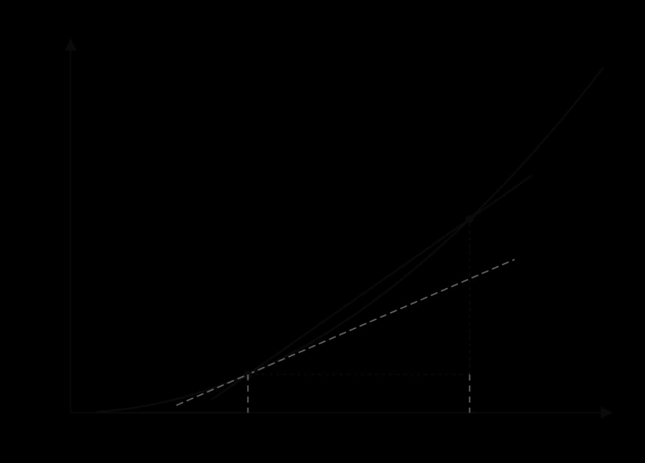
The diagram of the difference quotient shows why it works: the secant PQ has rise $f(a + h) - f(a)$ and run $h$, so its gradient is the difference quotient. Three versions are used for estimates.

For a curve that bends, the forward difference overestimates the gradient on one side and the backward difference underestimates it, so the symmetric difference, which balances the two, is usually much more accurate for the same $h$. For $y = x^2$ at $x = 3$ with $h = 1$, the forward difference gives 7, the backward difference 5, and the symmetric difference $\frac{16 - 4}{2} = 6$, the exact value. GDCs use the symmetric difference with a very small $h$ for their numerical derivative.

The derivative

The gradient function

Repeating the secant method for $y = x^2$ at other points gives a gradient at each one. The results show a pattern.

Each gradient is twice the $x$-coordinate, so the gradient of $y = x^2$ at any point is $2x$. This rule is itself a function: input any $x$, and it outputs the gradient of the curve there. It is called the gradient function, or derivative, of $x^2$. Spotting such a pattern and testing it with further values is how the general rules of differentiation in subtopic 5.3 are discovered; the pattern $2x$ is an example of generalisation.

Plotting the curve and its gradient function on the same axes shows how they are related. Where $y = x^2$ slopes down (for $x < 0$) the gradient function is negative; at the bottom of the curve, where the tangent is horizontal, the gradient function is 0; and where the curve climbs more and more steeply, the gradient function takes larger and larger positive values.

The value of the derivative at one point is a number, such as $f'(3) = 6$; the derivative itself is a function, such as $f'(x) = 2x$. Both are called "the derivative", and the context shows which is meant: "find $f'(x)$" asks for the function, while "find $f'(3)$" asks for one number, the gradient at $x = 3$.

Notation for the derivative

Calculus was developed independently in the late seventeenth century by Isaac Newton in England and Gottfried Wilhelm Leibniz in Germany. Two notations for the derivative are in common use today: Leibniz's notation, which keeps track of the variables, and the shorter prime notation, named after Joseph-Louis Lagrange, who used it about a century later.

The symbol $\frac{\mathrm{d}y}{\mathrm{d}x}$ is read "d y by d x" or "the derivative of $y$ with respect to $x$". It grew out of $\frac{\Delta y}{\Delta x}$, the change in $y$ over the change in $x$ for a secant, with the "d" standing for a change that has been made vanishingly small. It is a single symbol for a limit, and the two "d"s cannot be cancelled as they could in an ordinary fraction.

The letters change with the context. Any two related quantities have a derivative, and the notation shows which is which.

The value of a derivative at a particular point can be written in several ways. For $y = x^2$ at $x = 3$, all of $f'(3) = 6$, $\frac{\mathrm{d}y}{\mathrm{d}x} = 6$ when $x = 3$, and $\left.\frac{\mathrm{d}y}{\mathrm{d}x}\right|_{x = 3} = 6$ mean the same thing.

The derivative as a rate of change

The gradient of a graph and the rate of change of a quantity are the same thing seen in two ways. If $y$ is plotted against $x$, the gradient at a point says how many units $y$ increases for each unit increase in $x$ at that point, which is exactly the rate at which $y$ is changing with respect to $x$.

The average rate of change over an interval is the gradient of a secant. The rate of change at one value of the input, with no interval at all, is the gradient of the tangent there, which is the value of the derivative.

A speedometer gives instantaneous speed; a journey's distance divided by its time gives average speed. Both are rates of change of distance with respect to time. An average rate describes a whole interval, while an instantaneous rate describes a single moment and may differ greatly from the average.

Interpreting a derivative in context

A good interpretation of a derivative value contains four pieces of information: which quantity is changing, whether it is increasing or decreasing (the sign), how fast (the size, with units), and at which value of the input. A derivative of 0 means that, at that instant, the quantity is neither increasing nor decreasing.

The units follow directly from the notation: the units of the quantity on top divided by the units of the variable underneath. A rate of change keeps the context's wording, so "the volume increases at 314 cm³ per cm of radius" is a full interpretation, while "the gradient is 314" is not.

Average and instantaneous rates in real data

Measurements of carbon dioxide at the Mauna Loa Observatory in Hawaii, the series known as the Keeling Curve, rose from 313 parts per million (ppm) in March 1958 to 406 ppm in November 2018. The average rate of change over those 60 years and 8 months is

The current rate of increase is about 2.48 ppm per year. The secant over six decades gives a single average for the whole period, although the curve has become steeper over time. An instantaneous rate near 2018 is much larger than the long-run average, because the rate of change has itself been increasing.

Source: Keeling Curve measurements, Scripps Institution of Oceanography and NOAA Global Monitoring Laboratory, as summarised on Wikipedia "Keeling Curve", 2026.

Marginal cost

In economics, the derivative of a cost function is called the marginal cost. If $C(x)$ is the total cost of producing $x$ items, then $C'(x)$ is the rate at which the cost increases per extra item when $x$ items are being made. Because one item is a small change compared with hundreds, $C'(x)$ is very close to the cost of producing the next item, $C(x + 1) - C(x)$, which is a difference quotient with $h = 1$.

Marginal cost is used to decide whether producing more is worthwhile. If making one more item costs less than the price it sells for, the extra item adds to the profit. The cost function itself, and the related revenue and profit functions, are introduced in subtopic 2.5.

Estimating a derivative

Three methods give a value for a derivative without any rules of differentiation: difference quotients from a table, a tangent drawn on a graph, and the GDC's numerical derivative. All three are estimates of the same limit.

From a table of data

When a quantity is known only at certain times, its rate of change at a time in the table is estimated with a difference quotient using neighbouring entries. The symmetric difference, with one entry on each side, is the most reliable choice when it is available. Data collected more often (smaller $h$) give better estimates, which is the limit idea applied to real measurements.

The depth of water, $d$ cm, in a draining tank is measured every 5 minutes, with the results in the table of depths.

From a graph by drawing a tangent

On an accurate graph, the gradient at a point is estimated by drawing the tangent there with a ruler, so that it touches the curve and has the same direction as the curve at the point, then choosing two points far apart on the tangent and using the gradient formula. Points far apart reduce the effect of small errors in reading the scale. The answer is an estimate whose accuracy depends on the drawing, so two students may get slightly different values.

With the GDC

A GDC finds the derivative at a point numerically. It does not differentiate algebraically; it evaluates a symmetric difference quotient with a tiny $h$, which for the smooth functions used in modelling is accurate to many decimal places. The method works for any function the GDC can evaluate, including models that cannot yet be differentiated by hand.

• On the home screen: use the numerical derivative command. On a TI-84 Plus CE: MATH → 8:nDeriv(, then enter the function, the variable and the value, for example $\frac{\mathrm{d}}{\mathrm{d}x}(x^2)\big|_{x=3}$. On a Casio fx-CG50, in the Run-Matrix menu: OPTN → CALC → d/dx. On a TI-Nspire: menu → Calculus → Numerical Derivative at a Point.

• On the graph screen: graph the function, then use the derivative-at-a-point tool. On a TI-84 Plus CE: 2nd TRACE (CALC) → 6:dy/dx, then type the $x$-value.

• The whole gradient function: graph $y = f(x)$ together with the numerical derivative entered as a second function (on a TI-84, $\text{Y2} = \text{nDeriv}(\text{Y1}, X, X)$). The second graph is the gradient function, and its features can be found with the usual graph tools.

Reading the derivative from graphs

The graph of a function contains enough information to describe its gradient function, without any formula. Three features of $f'$ can be read from the graph of $f$ directly.

• The sign of $f'(x)$. Where the graph rises from left to right, the tangent has a positive gradient, so $f'(x) > 0$. Where it falls, $f'(x) < 0$. Where the tangent is horizontal, $f'(x) = 0$.

• The size of $f'(x)$. The steeper the graph, the larger the size of the gradient, $|f'(x)|$, whether the graph is rising or falling.

• Where the gradient is extreme. The graph is steepest uphill where $f'$ takes its greatest value, and steepest downhill where $f'$ takes its least (most negative) value.

The sign of the derivative and its link to increasing and decreasing functions are developed in subtopic 5.2, Increasing and decreasing functions, and the points where $f'(x) = 0$ in subtopic 5.6, Stationary points.

Steepness is the size of the gradient

"Steepest" refers to the size of the gradient, whatever its sign. A road that falls 30 m for every 100 m travelled is steeper than one that rises 20 m for every 100 m, even though −0.3 is less than 0.2. On a graph of a derivative, the steepest point of the original function is where $|f'(x)|$ is greatest, which may be at the lowest point of the derivative graph rather than the highest.

A ski run gives a clear example. The graph of the gradient function $h'(x)$ of the slope's height $h(x)$, with its zeros and extreme values marked, is enough to describe the whole shape of the run.

Each zero of $h'$ lines up with a horizontal tangent on the ski run, and each extreme value of $h'$ lines up with a part of the run that is locally steepest. Reading the two graphs together, with their $x$-axes lined up, is the quickest way to move between a function and its derivative.

Sketching a gradient function from a graph

The same reading works in reverse: from the graph of $f$, a sketch of $f'$ can be built up without a formula.

1. Mark the $x$-values where the tangent to $f$ is horizontal. The graph of $f'$ crosses or touches the $x$-axis at each of them.

2. On each interval between those points, decide whether $f$ is rising or falling. Draw $f'$ above the axis where $f$ rises and below it where $f$ falls.

3. Find where $f$ is steepest on each interval. That is where $f'$ is furthest from the axis (a local maximum or minimum of $f'$).

4. Check the ends: if $f$ keeps getting steeper, $f'$ keeps moving away from the axis.

Case study: Usain Bolt's 100 m world record

At the 2009 World Championships in Berlin, Usain Bolt ran 100 m in 9.58 seconds, a world record. A biomechanics team measured his times at several points along the track. Distance as a function of time gives a real example of a curve whose gradient, his speed, changes throughout the race.

Source: IAAF, Biomechanical analysis of the men's 100 m semi-final and final, 12th IAAF World Championships in Athletics, Berlin, 2009. Times are from the starting gun, so they include his reaction time of 0.146 s.

Average speed for the whole race

The average speed is the gradient of the secant from the start to the finish on the distance–time graph:

This number describes the whole race, but Bolt was never running at a steady 10.4 m s⁻¹. He started from rest and was much slower than that for the first 20 m and faster than that for most of the rest of the race.

Average speeds over each section

Each pair of neighbouring measurements gives a secant gradient, the average speed over that section.

The section speeds show the shape of the race. Bolt accelerated hard over the first 40 m, reached his highest average speed between 60 m and 80 m, and slowed slightly over the last 20 m. The graph of distance against time is therefore a curve that gets steeper and then very slightly less steep.

Estimating his speed at an instant

His speed at the moment he passed 60 m is an instantaneous rate of change, $\frac{\mathrm{d}s}{\mathrm{d}t}$ at $t = 6.31$. The data allow three estimates using the neighbouring measurements at 40 m and 80 m.

The best estimate from the data is about 12.2 m s⁻¹ (44 km/h), the symmetric difference. These estimates cannot be improved by making $h$ smaller, because the measurements stop at intervals of 20 m. Finer timing (such as video at many frames a second, or laser measurements) would give secants over shorter intervals and so estimates closer to the true instantaneous speed.

Interpreting the sprint data

• An average rate (10.4 m s⁻¹) can be very different from the rate at an instant (about 12.2 m s⁻¹ at 60 m, under 7 m s⁻¹ on average over the first 20 m).

• With real data, the derivative is always estimated from secants, and the size of the interval limits the accuracy.

• The derivative of distance with respect to time is speed, so the gradient of a distance–time graph at a point has units of m s⁻¹.

• The model of a smooth curve through the points is an assumption: an athlete's speed changes slightly within every stride, which no table of 20 m splits can show.

Exam focus

Limits and the meaning of the derivative are rarely examined on their own. They appear as the opening parts of longer questions on Paper 1 and Paper 2, usually for 1 to 3 marks each, before the question moves on to differentiation (subtopic 5.3), tangents (5.4), stationary points (5.6) or integration (5.5). The command terms are write down, estimate, find, interpret, identify and sketch.

The recurring question shapes are:

• interpret a derivative value such as $\frac{\mathrm{d}P}{\mathrm{d}t} = -4$ in context, naming the quantity, whether it increases or decreases, and the units;

• estimate a rate of change from a table of data with a difference quotient, showing the quotient;

• find a derivative at a point with the GDC, then interpret it;

• identify from the graph of $f'$ where $f$ is steepest, highest or lowest, and sketch $f$ from $f'$ or $f'$ from $f$;

• write down the long-run value of a model (a limit as $t \to \infty$) and interpret it, or use a given limit to sketch a curve with its asymptote.

A question on the graph of a derivative usually rewards a careful reading of the words "steepest", "greatest rate" and "highest". Writing $|f'(x)|$ greatest, or "$f'$ changes from positive to negative", next to the answer shows the reasoning.

When a part asks for an estimate from a table, write the difference quotient with the numbers substituted before the answer, for example $\frac{63 - 98}{15 - 5}$. The method mark is for the quotient, and an answer alone cannot show which entries were used. If a later part uses a wrong earlier answer correctly, follow-through marks are available, so a part should never be left blank because an earlier part went wrong.

Practice questions

1. By completing a table of values on both sides of $x = 1$, estimate $\lim_{x \to 1} \frac{x^5 - 1}{x - 1}$. [3]

2. The number of fish in a lake, $N$, $t$ years after restocking, is modelled by $N(t) = 800 - 650 \times 0.85^{t}$. Write down the number of fish at $t = 0$

3. For $f(x) = 2x^2$, calculate the gradient of the secant from $x = 1$ to $x = 1 + h$

4. An app had 30,000 downloads 4 weeks after launch and 81,000 downloads 10 weeks after launch. Find the average rate of change of the number of downloads between weeks 4 and 10, with units. [2]

5. (a) A cyclist's distance from home is $s$ metres after $t$ seconds. Write down the units of $\frac{\mathrm{d}s}{\mathrm{d}t}$. [1] (b) The temperature of a cup of soup, $T$

6. The temperature in an oven, $T$ °C, is recorded every 3 minutes after it is switched on: 20 ($t = 0$), 74 ($t = 3$), 115 ($t = 6$), 146 ($t = 9$

7. Let $g(x) = 3 \times 1.2^{x} - x$. (a) Find $g'(2)$

8. For a function $f$, $f'(1) = 3.2$, $f'(2) = -0.5$

9. The cost, in dollars, of making $x$ ceramic mugs is $C(x) = 500 + 20x - 0.01x^2$, $0 \le x \le 800$

Summary

• $\lim_{x \to a} f(x) = L$ means $f(x)$ gets as close to $L$ as required when $x$ is close enough to $a$, from both sides; the value at $a$ itself does not matter. Limits are estimated from tables (values on both sides) or graphs.

• A limit as $x \to \infty$ gives the long-run value of a model, seen as a horizontal asymptote.

• The gradient of a secant, $\frac{f(b) - f(a)}{b - a}$, is the average rate of change over an interval.

• The gradient of a curve at a point is the gradient of its tangent: the limit of the secant gradients $\frac{f(a + h) - f(a)}{h}$ as $h \to 0$.

• The derivative $f'(x)$ or $\frac{\mathrm{d}y}{\mathrm{d}x}$ is the gradient function: it gives the gradient, and the instantaneous rate of change, at every $x$

• Units of a derivative: units of the top quantity per unit of the bottom variable. An interpretation states the quantity, increasing or decreasing, the rate with units, and when.

• Derivatives are estimated from data with difference quotients (the symmetric difference is usually best), from graphs by drawing tangents, and with the GDC's numerical derivative ("$f'(2) = 6$ (GDC)").

• Marginal cost $C'(x)$ approximates the cost of producing one more item.

• On the graph of $f'$: positive values mean $f$ rises, negative values mean $f$ falls, zeros mean horizontal tangents, and $f$ is steepest where $|f'(x)|$

Self-check

• To do:

  I can build a table of values on both sides of a point and estimate a limit to 3 significant figures.

• To do:

  I can explain why a function can have a limit at a point where it is undefined.

• To do:

  I can find the long-run value of a model as a limit and interpret it.

• To do:

  I can calculate the gradient of a secant and interpret it as an average rate of change with units.

• To do:

  I can explain how secant gradients approach the gradient of the tangent as the second point moves towards the first.

• To do:

  I can write forward, backward and symmetric difference quotients and say which is usually most accurate.

• To do:

  I can explain the difference between $f(a)$, $f'(a)$ and $f'(x)$.

• To do:

  I can read and write $\frac{\mathrm{d}y}{\mathrm{d}x}$, $f'(x)$, $\frac{\mathrm{d}V}{\mathrm{d}r}$

• To do:

  I can interpret a derivative value in context, including its sign.

• To do:

  I can find a derivative at a point with my GDC and write down what I found.

• To do:

  I can estimate a rate of change from a table of real data.

• To do:

  I can explain what marginal cost means and estimate it.

• To do:

  I can identify where a function is steepest from the graph of its derivative, using $|f'(x)|$.

• To do:

  I can sketch the gradient function from the graph of a function.

A second point $Q(x,\ f(x))$ also lies on the graph of $f$. The following table shows the gradient of the chord $PQ$ for different values of $x$.

1. (a)

   Find the value of $p$ and the value of $q$. Give your answers correct to five decimal places where necessary.

   [3]3 marks

   Markscheme (a)

   attempt to find the gradient of a chord, $\dfrac{f(x) - 4}{x - 2}$ (M1)

   $p = \dfrac{0.5(2.1)^3 - 4}{2.1 - 2} = 6.305$ A1

   $q = \dfrac{0.5(2.001)^3 - 4}{2.001 - 2} = 6.00300$ $(6.0030005)$

   Note: Accept $q = 6.003$.

   [3 marks]

2. (b)

   Use the table to estimate the gradient of the tangent to the graph of $f$ at $P$.

   [1]1 mark

   Markscheme (b)

   $6$ A1

   [1 mark]

3. (c)

   Write down the value of $f'(2)$.

   [1]1 mark

   Markscheme (c)

   $f'(2) = 6$ A1

   Note: Follow through from their answer to part (b).

From below the values increase towards 3; from above they decrease towards 3. The two sides agree, so

The estimate is supported by the pattern: at a distance of 0.001 from 1, both values are within 0.004 of 3.

(b) Use the GDC's table for large values of $t$:

Because $0.82^{t} \to 0$ as $t \to \infty$, the values approach 450:

(c) In the long run the number of subscribers levels off at about 450,000. The model predicts that the service never quite reaches 450,000 subscribers, so the limit is a ceiling for the model rather than a value that is reached.

Between edge lengths of 2 cm and 2.1 cm, the volume increases at an average rate of 12.61 cm³ per cm of edge length.

(b)

(c) From the right the gradients decrease towards 12, and from the left they increase towards 12. The gradient of $V = x^3$ at $x = 2$ is 12 (cm³ per cm). When the edge is 2 cm, the volume is increasing at 12 cm³ for each centimetre of extra edge length.

The volume increases by about 31.4 cm³. As a check, the exact volumes are $\frac{4}{3}\pi(5.1)^3 - \frac{4}{3}\pi(5)^3 = 32.0$ cm³ to 3 significant figures; the estimate is slightly low because the rate itself increases as the radius grows.

Producing the 301st frame costs an extra $15.01 (to the nearest cent).

(b) Using the GDC's numerical derivative of $C(x)$ at $x = 300$: $C'(300) = 15$.

(c) When 300 frames a week are being produced, the total cost is increasing at $15 per extra frame: this is the marginal cost at $x = 300$. It is very close to the actual cost of the 301st frame, $15.005, because the cost function bends only slightly over an interval of one frame. Marginal cost is a quick approximation to the cost of one more unit.

(b) Using the GDC's numerical derivative at $t = 5$: $h'(5) = 5.13$ (3 s.f.).

(c) Five weeks after planting out, the sunflower is growing at about 5.13 cm per week. This is faster than the average over the first 10 weeks because growth is slow at the start (the plant is small) and speeds up in the middle of the period: the average combines slow and fast weeks, while $h'(5)$ is the rate at one instant in the fast phase.

(b) The skier travels uphill where the height increases, which is where $h'(x) > 0$: for $250 < x < 380$.

(c) The graph of $h$ starts at (0, 80) with a horizontal tangent, falls (steepest near $x = 87$) to a local minimum at $x = 250$, rises gently to a local maximum at $x = 380$, then falls again, most steeply near $x = 521$, to finish at (600, 0) with a horizontal tangent.

The gradient function is U-shaped, crossing the $x$-axis at 1 and 3 with its minimum at $x = 2$. (The $y$-coordinates 5 and 1 of the turning points of $f$ play no part in the sketch of $f'$.)

$= 8.4$ mg/L per hour A1

(c) GDC numerical derivative at $t = 1$ (M1)

$C'(1) = 13.5$ $(13.5098\ldots)$ A1

(d) one hour after taking the medicine, the concentration is increasing A1

at a rate of 13.5 mg/L per hour A1

Note: award at most A1A0 if the units or the reference to time are missing.

(e) the concentration is decreasing (at 3.07 mg/L per hour) A1

(f) 0 A1

in the long run the medicine is (almost) completely removed from the blood / the concentration approaches zero A1

Total [10]

[1 mark]