5.6 Stationary points · IB Maths AI | Augment Education
5.6 Stationary points
Find where the gradient of a curve is zero by solving f′(x) = 0 by hand or with a GDC, classify local maxima and minima with the first derivative test, and find greatest and least values on a domain.
IB Mathematics: Applications and Interpretation
Part of 5 Calculus
SL and HL
Key terms introduced here
Each is in the Maths AI glossary, with every other term in the subject.
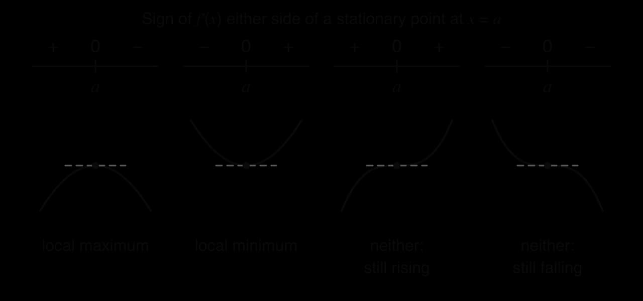
A method of finding the nature of a stationary point at x=a from the sign of f′(x) just to the left and just to the right of a: a change from positive to negative shows a local maximum, a change from negative to positive shows a local minimum, and no change of sign shows neither.
Find the coordinates of the stationary points of a function, using f (not f′) for the y-coordinate.
Determine whether a stationary point is a local maximum or a local minimum, using the sign of f′(x) on either side or the graph of the function.
Use technology to generate the graph of f′(x) from f(x) and to find its zeros.
Explain why a local maximum or minimum need not be the greatest or least value of a function on a given domain, and find the greatest and least values by checking the end points.
Use the values at stationary points to find the range of a function and the number of solutions of f(x)=k.
Find unknown coefficients of a function from information about its stationary points.
Interpret stationary points of a model in context, including the peak of a real data set.
Introduction
A curve that rises and then falls must level off for an instant at the top. At that instant its tangent is horizontal and its gradient is zero. Points like this, where the derivative equals zero, are called stationary points, and they mark the tops of hills and the bottoms of valleys on the graph of a function. Finding them gives the largest and smallest values of a quantity in a model, which is often the reason the model was built.
The method joins together the ideas of subtopics 5.1 to 5.3. The derivative gives the gradient of the curve at every point, so the stationary points are the solutions of the equation f′(x)=0. The sign of the derivative on either side then shows whether the curve has reached a peak or a trough. The same steps locate the highest point of a model of a bridge arch and the week in which new infections in an epidemic stopped rising.
Where the gradient of a curve is zero
The gradient of a curve at a point is the gradient of the tangent there, and the derivative f′(x) gives that gradient for every value of x (subtopic 5.1). When the derivative is positive the curve is rising from left to right, and when it is negative the curve is falling (subtopic 5.2). Between a stretch where a smooth curve rises and a stretch where it falls, the gradient changes from positive to negative, and at the point where it changes it is exactly zero.
The equation of a horizontal tangent has the form y=c, where c is the y-coordinate of the point of contact. For the curve y=x3−3x the derivative is dxdy=3x2−3, which is zero when x=1 or x=−1. The points of the curve there are (1,−2) and (−1,2), and the graph of y=x3−3x shows the horizontal tangents y=2 and y=−2 touching the curve at its top and bottom.
y = x³ − 3x
At (−1, 2) and (1, −2) the tangent to y = x³ − 3x is horizontal: the gradient is zero there, and these are the top of the hump and the bottom of the dip.
The name comes from the idea of a quantity that is changing. If y is a height, a temperature or a population and x is time, then f′(x) is the rate of change of y, and a stationary point is an instant at which y is momentarily not changing: neither increasing nor decreasing. The value f(a) at a stationary point is called a stationary value.
Why the gradient is zero at a smooth peak or trough
Two arguments lead to the same result. The first is geometric. At the top of a smooth hump every nearby point of the curve lies below the point at the top. Any line through the top with a positive gradient would cut into the curve on its right, and any line with a negative gradient would cut into it on the left, so the only line that just touches the curve there is horizontal.
The second argument uses the sign of the derivative. To the left of a smooth peak the curve rises, so f′(x)>0; to the right it falls, so f′(x)<0. For a polynomial the derivative is itself a polynomial, whose graph has no gaps, so it cannot change from positive to negative without passing through zero. At the peak, therefore, f′(x)=0. The same reasoning applied to a trough, where the gradient changes from negative to positive, gives the same equation.
at a smooth local maximum or local minimum at x=a:f′(a)=0
The two kinds of point are the local maximum and the local minimum met without calculus in subtopic 2.4, Key features of graphs. Calculus adds an exact way to find them: instead of searching along a graph, the equation f′(x)=0 is solved.
Stationary points that are not turning points
The reasoning works in one direction only. Every smooth peak or trough has f′(x)=0, but a point with f′(x)=0 need not be a peak or a trough. The curve y=x3 has derivative 3x2, which is zero at x=0, so (0,0) is a stationary point. Yet the curve rises on both sides of the origin: it flattens for an instant and then keeps rising. The stationary point at the origin is not a turning point, because the curve does not turn.
Stationary points of this third kind are called stationary points of inflexion. The first derivative test identifies them as "neither a maximum nor a minimum", and HL subtopic 5.10 studies them in full.
Solving f′(x) = 0
Every stationary point problem follows the same three steps. The first is to differentiate, using the power rule of subtopic 5.3. The second is to solve f′(x)=0 for x. The third is to substitute each solution into the original functionf to find the y-coordinate.
Differentiate: find f′(x).
Solve f′(x)=0, by hand or with technology. Keep only solutions in the domain.
Substitute each solution into f(x) to find the y-coordinate of each stationary point.
For a cubic function the derivative is a quadratic, so there are at most two stationary points; a quadratic derivative with no real roots means the cubic has none at all. For a quartic the derivative is a cubic, giving up to three. In general a polynomial of degree n has at most n−1 stationary points, because its derivative has degree n−1.
f(x)
Degree of f′(x)
Most stationary points
Example
quadratic
1 (linear)
1
x2−4x: one, at x=2
cubic
2 (quadratic)
2
x3−3x: two; x3+x: none
quartic
3 (cubic)
3
x4−8x2: three
Solving by hand
When the derivative is linear or a quadratic that factorises, the equation f′(x)=0 can be solved quickly by hand. Taking out a common factor first keeps the numbers small.
The function in the worked example and its derivative are drawn on the same axes in the graph of f and f′. The zeros of f′ at x=−1 and x=4 sit directly beneath the hump and the dip of f. Where the graph of f′ is above the x-axis, f is rising; where it is below, f is falling.
y = f(x)
y = f′(x)
The zeros of f′ (x = −1 and x = 4) line up with the stationary points of f; f′ is positive where f rises and negative where f falls.
Solving with technology
Many derivatives do not factorise, and the equation f′(x)=0 is then solved with the GDC. There are three ways, and the derivative may be found by hand or produced by the GDC itself.
Polynomial root finder. When f′(x) is a quadratic or cubic, enter its coefficients into the GDC's polynomial equation solver (subtopic 1.8). It gives every real root at once.
Graph the derivative and find its zeros. Enter f′(x) as a function, either typed by hand or generated by the GDC's numerical derivative (on a TI-84 Plus CE, MATH → 8: nDeriv(, entered as Y2 = nDeriv(Y1, X, X) when f is in Y1; other models have a dxd template). Then use the zero (root) tool on its graph.
Graph the function and use the maximum and minimum tools. On a TI-84 Plus CE these are 2ndTRACE (CALC) → 4: maximum or 3: minimum; on a Casio fx-CG50 they are SHIFTF5 (G-SOLVE) → MAX and MIN. Each tool asks for a left bound and a right bound on either side of the turning point and returns both coordinates.
The first two methods solve the equation f′(x)=0 directly. The third finds the turning points without the derivative at all, which makes it a good check, but it cannot be used when a question asks for the derivative to be used, and it does not find a stationary point that is not a turning point (the curve of y=x3 has no maximum or minimum for the tool to find).
Derivatives with negative powers
Functions such as f(x)=x2+x54 appear often in applications, because a fixed area or volume divided by a length produces a term in x1. The method is the same, but the term must first be written as a negative integer power, 54x−1, before the power rule is applied. The equation f′(x)=0 then contains a fraction, and multiplying both sides by a power of x clears it.
Local maximum and minimum points
Solving f′(x)=0 locates the stationary points but does not say what kind each one is. The kind of point is its nature.
The nature can be read from a graph of the function drawn on the GDC: a hump is a local maximum and a dip is a local minimum. When a reason based on the derivative is needed, the sign of f′(x) on each side of the point decides it.
The first derivative test
A local maximum is a point where the curve stops rising and starts falling. In terms of the derivative, f′(x) is positive just to the left of the point, zero at it, and negative just to the right. A local minimum is the reverse: negative, zero, positive. If the sign is the same on both sides, the curve has flattened for an instant without turning, and the point is neither.
The four possible patterns appear in the figure of sign diagrams, each with a sketch of the shape of the curve it produces. A sign diagram records the signs on a number line with the stationary values of x marked.
The pattern of signs of f′(x) either side of x = a decides the nature: + then − is a local maximum, − then + is a local minimum, and the same sign on both sides is neither.
Sign of f′(x) just left of a
f′(a)
Sign of f′(x) just right of a
Nature of the stationary point
+
0
−
local maximum
−
0
+
local minimum
+
0
+
neither (the curve keeps rising)
−
0
−
neither (the curve keeps falling)
Choosing the test points
The test values of x must lie between the stationary point being tested and the next stationary point on each side. Between two neighbouring zeros of a polynomial derivative, f′(x) keeps one sign throughout, so any single value in the interval shows the sign of the whole interval. A test value chosen beyond the next stationary point may show the wrong sign. Values that make the arithmetic easy, such as whole numbers or 0, are the best choices.
Using the graph to decide the nature
A sketch of y=f(x) from the GDC is also a valid justification, provided it is labelled: the stationary point, its coordinates and the shape on either side. A sketch of y=f′(x) works as well: if the graph of the derivative crosses the x-axis from above to below at x=a, the sign of f′ goes from positive to negative and the point is a local maximum. A graph of f′ that only touches the axis without crossing it shows a stationary point that is neither.
YouTube
Khan Academy, “Finding relative extrema (first derivative test)”: watch how the sign of the derivative on each side of each critical point is tested to classify it as a relative maximum or minimum.
The video uses the American names "relative extremum" for a local maximum or minimum and "critical point" for a point where the derivative is zero; the method is the same first derivative test.
Greatest and least values on a domain
A local maximum is higher than the points next to it, but it need not be the highest point of the graph. A function defined on a restricted domain, such as 0≤t≤10, can reach a larger value at an end of the domain, where the curve simply stops while still rising.
On a closed domain a≤x≤b, the greatest and least values of a polynomial can only occur at stationary points or at the end points x=a and x=b. Everywhere else the curve is either rising or falling, so a neighbouring point is higher and another is lower. This gives a reliable method.
Find the stationary points that lie inside the domain.
Evaluate the function at each of them and at both end points.
The largest of these values is the global maximum and the smallest is the global minimum.
The range of the function on the domain then runs from the global minimum to the global maximum. This is how the range of a function (subtopic 2.2) is found with calculus.
The graph of the profit model shows why the end point wins: the curve is still rising when the domain ends at t=10.
P(t)
The local maximum at t = 2 is not the greatest value on 0 ≤ t ≤ 10: the end point (10, 10) is higher. The local minimum (7, 0.55) is also the global minimum.
The number of solutions of f(x) = k
The stationary values also show how many times a horizontal line y=k meets a curve, which is the number of solutions of the equation f(x)=k (subtopic 1.8). A cubic with a local maximum value M and a local minimum value m rises, falls and rises again (when its x3 coefficient is positive). A horizontal line strictly between m and M crosses all three parts of the curve, a line at exactly m or M touches one turning point and crosses one other part, and any other line crosses only once.
Value of k
Number of solutions of f(x)=k for a cubic with local max value M and local min value m
m<k<M
3
k=m or k=M
2
k<m or k>M
1
Finding unknown coefficients from stationary points
Information about a stationary point gives equations for unknown parameters in a function. "The graph has a stationary point at x=a" means f′(a)=0; "the graph passes through (a,b)" means f(a)=b. A stationary point with both coordinates given supplies both equations at once.
When two coefficients are unknown, two conditions are needed, and they form a system of linear equations that can be solved by hand or with the GDC's simultaneous equation solver.
Stationary points in context
In a model, the stationary point answers a question in the language of the situation: the highest point of a structure, the moment a quantity stops growing, the price at which demand peaks. The answer must be given in that language, with units, and checked against the reasonable domain of the model, since a solution of f′(x)=0 outside it has no meaning.
The arch of the Sydney Harbour Bridge
The Sydney Harbour Bridge has a steel arch with a span of 504 m between its abutments and a summit 134 m above mean sea level. The real arch is not exactly a parabola, but a quadratic model shows how calculus finds the highest point.
Source of the bridge dimensions: Wikipedia, "Sydney Harbour Bridge", accessed 2026.
The model fits the two facts it was built from, the span and the summit, and calculus confirms that the vertex of the parabola is the highest point. The real arch rests on hinges at its ends and its curve is not exactly quadratic, so the gradient near the abutments is an estimate only.
Case study: the peak of Italy's first COVID-19 wave
Italy was the first European country hit hard by COVID-19 in early 2020. The table gives the number of new confirmed cases reported in each week from the week dated 8 March 2020 to the week dated 10 May 2020, with t the number of weeks after the week dated 1 March 2020.
t
1
2
3
4
5
6
7
8
9
10
Week dated
8 Mar
15 Mar
22 Mar
29 Mar
5 Apr
12 Apr
19 Apr
26 Apr
3 May
10 May
New cases
4,755
15,274
32,421
38,894
32,160
27,639
23,654
19,426
13,977
8,940
Source: World Health Organization weekly COVID-19 data, as compiled at ourworldindata.org (owid/covid-19-data), accessed 2026.
A cubic function fitted to the ten points by least squares with technology, with coefficients rounded to 4 significant figures, is
N(t)=228.3t3−5048t2+30930t−23160,1≤t≤10,
where N is the number of new cases in a week. The week in which new cases stopped rising is modelled by the local maximum of N.
N′(t)N′(t)=0=684.9t2−10096t+30930⇒t=4.343… or t=10.397…(GDC)
The first derivative test classifies the two points: N′(4)=1504.4>0 and N′(5)=−2427.5<0, so t=4.343 is a local maximum, with N(4.343…)=34656.8… The model puts the peak of the wave about 4.3 weeks after the week dated 1 March, between the weeks dated 29 March and 5 April, at about 34,700 new cases a week. The data agree on the timing: the largest weekly count, 38,894, is in the week dated 29 March (t=4).
N(t), fitted cubic
model beyond the data
The cubic's local maximum (t ≈ 4.34) matches the timing of the real peak but underestimates its height; its local minimum near t = 10.4 predicts a rise that never happened. Data: WHO, via ourworldindata.org.
The second stationary point, a local minimum at t≈10.4, lies just beyond the data. The cubic predicts that cases would start rising again after mid-May 2020, but the reported weekly counts kept falling: 6,492 in the week dated 17 May and 4,567 in the week dated 24 May. That turning point is a feature of the cubic, which must eventually rise because its t3 term dominates, and not a feature of the epidemic. The cubic is therefore useful for locating the peak within the ten weeks of data, but it should not be used to predict the number of cases after them.
Three further limitations affect the interpretation. Confirmed cases depend on how much testing is done, so the real number of infections was higher, and early in the wave testing was limited. Weekly totals hide day-to-day changes, so "the peak" is only located to within a week. A polynomial has no mechanism behind it; epidemic models built from how a disease spreads, such as the SIR model of HL subtopic 5.16, explain why the peak comes when it does.
Exam focus
Stationary points are examined on both papers, usually as two to five parts inside a longer question on a cubic or a model: profit, the height of a structure, a population, a volume. Paper 1 tends to give a function and ask for its derivative and stationary points (5–7 marks); Paper 2 builds a context around it, then asks for the maximum, the range, or the number of solutions of an equation, and often moves on to optimisation (subtopic 5.7). The command terms are find (show working), write down (little working, often a GDC value), show that (work forwards to a given result), hence and use your answer to (the derivative must be used), determine and justify (a reason is needed for the nature or for an end point).
Markschemes follow a regular pattern: (M1) for setting the derivative equal to zero, (A1) for the x-value, (M1) for substituting it into the original function, A1 for the y-value. When the question says "hence" after asking for f′(x), an unsupported GDC maximum earns no marks; the equation f′(x)=0 must be seen. Read whether the question asks for "the coordinates", "the value of x" or "the maximum value": giving a pair when only y is asked, or only x when coordinates are asked, loses a mark.
The values in part (d) are found by substituting into the derivative: h′(50)=−0.0012(2500)+3+0.6=0.6 and h′(70)=−0.0012(4900)+4.2+0.6=−1.08. Part (f) depends on the end point: had the trail ended above 160 m, there would be only one such point.
Other recurring shapes are worth recognising: "the graph of f has a horizontal tangent at x=2; find a" (set f′(2)=0); "find the values of k for which f(x)=k has three solutions" (between the two stationary values); "state the interval on which the gradient is negative" (between the stationary points of a cubic with positive leading coefficient, using subtopic 5.2); "explain why the local maximum is not the greatest value" (an end point is higher).
Practice questions
Find the coordinates of the stationary points of the curve y=x3−12x+7. [4]
For the curve in question 1, use the first derivative test to determine the nature of each stationary point. [3]
Let f(x)=4x+x25, x>0. Findf′(x), and hencefind the coordinates of the stationary point of the graph of f. [5]
Let g(x)=0.2x3−x2−2.5x+6. Find the coordinates of the local maximum and local minimum points of the graph of g
The function f(x)=x3−6x2+px+1 has a stationary point at x=3
Let q(x)=x3−3x2−9x+10 for −2≤x≤6
For q(x)=x3−3x2−9x+10, x∈R
The concentration of a pollutant in a river, C mg per litre, t days after a spill, is modelled by C(t)=0.5t3−6t2+18t+4
The curve y=ax3+bx has a local maximum at (−1,4). Find the values of a and b
Answers
dxdy=3x2−12=0⇒x=±2. Points (−2,23) and (2,−9).
At x=−3: 15>0; at x=0: −12<0; at x=3
f′(x)=4−x225. 4−x225=0⇒x2=6.25⇒x=2.5
g′(x)=0.6x2−2x−2.5=0 (GDC) ⇒x=4.30190…
(a) f′(x)=3x2−12x+p; f′(3)=27−36+p=0⇒p=9
(a) q′(x)=3x2−6x−9=3(x−3)(x+1)
−17<k<15.
C′(t)=1.5t2−12t+18=1.5(t−2)(t−6)
dxdy=3ax2+b. Gradient zero at x=−1
Summary
A stationary point is a point where the gradient is zero: f′(a)=0, and the tangent there is horizontal.
To find stationary points: differentiate, solve f′(x)=0 (by hand or with the GDC), then substitute each x-value into f, not f′, for the y-coordinate.
Terms such as xa are rewritten as ax−1 before differentiating; multiplying through by a power of x clears the fractions in f′(x)=0
The GDC can solve f′(x)=0 with a polynomial root finder, by graphing f′ (typed or generated by the numerical derivative) and finding its zeros, or check the answer with the maximum and minimum tools.
First derivative test: f′ changes from + to − at a local maximum and from − to + at a local minimum; no change of sign means neither. Test points must lie between neighbouring stationary points.
A local maximum or minimum need not be the greatest or least value on a domain: compare the values at the stationary points and at both end points.
For a cubic with local maximum value M and local minimum value m, f(x)=k has three solutions when m<k<M
"Stationary point at x=a" gives the equation f′(a)=0; "passes through (a,b)" gives f(a)=b
In context, a stationary point is where a quantity momentarily stops changing; reject solutions outside the reasonable domain and check whether the model is valid there.
Self-check
To do:
I can explain why the gradient is zero at a smooth local maximum or minimum.
To do:
I can find f′(x) for a polynomial, including terms written as fractions such as x54.
To do:
I can solve f′(x)=0 by factorising when the derivative is a simple quadratic.
To do:
I can solve f′(x)=0 with the GDC's polynomial root finder and by finding the zeros of the graph of f′.
To do:
I can use the GDC's numerical derivative to draw the graph of f′ from f.
To do:
I can find the y-coordinate of a stationary point by substituting into f, not f′.
To do:
I can draw a sign diagram for f′ with test points in the right intervals.
To do:
I can use the first derivative test to classify each stationary point as a local maximum, a local minimum or neither.
To do:
I can recognise a stationary point that is not a turning point, such as the origin on y=x3.
To do:
I can find the greatest and least values of a function on a closed domain by checking the end points.
To do:
I can write down the range of a function on a domain from its greatest and least values.
To do:
I can find the values of k for which f(x)=k has one, two or three solutions.
To do:
I can find unknown coefficients from the position of a stationary point, setting up and solving the equations.
To do:
I can interpret a stationary point in context, with units, and reject solutions outside the reasonable domain.
To do:
I can write down the equation f′(x)=0 and its solution whenever a question says "hence" or "use your answer".
.
(a)
Find f′(x).
[2]2 marks
Markscheme (a)
f′(x)=6x2−18x−24A2
Note: Award A1 for two correct terms. Award A0 if there are extra terms.
[2 marks]
(b)
Find the coordinates of the two points on the graph of f where the gradient is zero.
[4]4 marks
Markscheme (b)
6x2−18x−24=0M1
x=−1
(c)
Determine the nature of the stationary point with x=−1. Justify your answer.
[2]2 marks
Markscheme (c)
EITHER
f′(−2)=36>0
Question 2 · AI-010936 marks
The function f is defined by f(x)=2x+x50, for x>0.
(a)
Find f′(x).
[2]2 marks
(b)
Use your answer to part (a) to find the coordinates of the local minimum point of the graph of f.
A check with the GDC: graphing y=2x3−9x2−24x+5 in the window −3≤x≤6, −120≤y≤40 shows a hump at x=−1 and a dip at x=4, at the heights found.
. The quadratic does not factorise, so the GDC is used.
GDC working. Polynomial root finder with coefficients a=1.5, b=−4, c=−3 gives
x=3.27698…orx=−0.610317…
(The quadratic formula gives the same values exactly: x=34±34.)
Substituting the stored, unrounded values into f:
f(3.27698…)=−9.71305…,f(−0.610317…)=4.97230…
The stationary points are (3.28,−9.71) and (−0.610,4.97).
As a check, the GDC's minimum tool on the graph of y=0.5x3−2x2−3x+4, with bounds x=2 and x=5, returns x=3.2769…, y=−9.7130…
(b) Set the derivative equal to zero and multiply both sides by x2 (allowed because x>0, so x2=0):
2x−x2542x3−54x3x=0=0=27=3
Then f(3)=32+354=9+18=27.
The stationary point is (3,27).
With technology, graphing y=2x−54/x2 for 0<x≤8 and using the zero tool gives x=3 as well.
:
4x3−16x4x(x2−4)4x(x−2)(x+2)=0=0=0
so x=−2, x=0 or x=2.
(b) The three stationary values split the number line into four intervals. One test value is chosen in each.
x
−3
−2
−1
0
1
2
3
g′(x)
−60
0
12
0
−12
0
60
sign
−
0
+
0
−
0
+
At x=−2 the sign changes from − to +: a local minimum, at (−2,−13), since g(−2)=16−32+3=−13.
At x=0 the sign changes from + to −: a local maximum, at (0,3).
At x=2 the sign changes from − to +: a local minimum, at (2,−13).
The graph of y=x4−8x2+3 on the GDC has the shape of a W, with two equal troughs and a central peak, which agrees.
.
Setting h′(x)=0 gives (x−2)2=0, which has only the solution x=2 (a repeated root). So there is exactly one stationary point.
h(2)=8−24+24−5=3, so the stationary point is (2,3).
(b) h′(1)=3(1−2)2=3>0 and h′(3)=3(3−2)2=3>0. The derivative is positive on both sides of x=2, so it does not change sign. The point (2,3) is neither a local maximum nor a local minimum: the curve rises, flattens for an instant at (2,3), and continues to rise.
In fact h′(x)=3(x−2)2 is a square times 3, so it is never negative: the function is increasing everywhere except at the single point x=2.
Both lie inside the domain.
(b) The first derivative test gives the nature: P′(1)=1.8>0, P′(3)=−1.2<0, P′(8)=1.8>0. So t=2 is a local maximum and t=7 a local minimum. Then evaluate P at the stationary points and at both end points.
t
0 (end point)
2 (local max)
7 (local min)
10 (end point)
P(t)
3
6.8
0.55
10
The greatest monthly profit is $10,000, at t=10, the end of the domain, not at the local maximum. The least is $550, at t=7.
(c) The range is 0.55≤P≤10 (thousand dollars).
The local maximum at t=2 is only the best month of the early period: profit dips afterwards, then recovers and overtakes it.
k=18
or
k=−107
.
y = f(x)
Any horizontal line strictly between y = −107 and y = 18 crosses the cubic three times; the lines through the turning points meet it only twice.
, so
f′(1)=0
:
3(1)2+2a(1)−152a−12a=0=0=6
(b) With a=6, f′(x)=3x2+12x−15=3(x2+4x−5)=3(x+5)(x−1), so the other stationary point is at x=−5.
f(−5)=−125+150+75+4=104, so the point is (−5,104).
Nature: f′(−6)=3(−1)(−7)=21>0 and f′(0)=−15<0, so the sign changes from positive to negative: a local maximum.
:
12a+4b=0
.
The point (2,−3) lies on the curve: 8a+4b+1=−3, that is, 8a+4b=−4.
(b) GDC working. Simultaneous equation solver with 12a+4b=0 and 8a+4b=−4 gives a=1, b=−3. (By hand, subtracting the equations gives 4a=4.)
So a=1 and b=−3, and the curve is y=x3−3x2+1.
(c) dxdy=3x2−6x=3x(x−2)=0 gives x=0 or x=2. At x=0, y=1, so the other stationary point is (0,1).
A sign check confirms the given information: the derivative is −3 at x=1 and 9 at x=3, so (2,−3) is indeed a local minimum.
(b) Expand first: h(x)=504kx−kx2. With k a constant, h′(x)=504k−2kx.
(c) Set h′(x)=0: 504k−2kx=0. Since k=0, divide by k: 504−2x=0, so x=252, the centre of the span, where h=134 m.
Nature: h′(x)=k(504−2x) with k>0 is positive for x<252 and negative for x>252, so the stationary point (252,134) is a local maximum: the summit of the arch.
(d) h′(0)=504k=63504504×134=1.0634…
The gradient is about 1.06: near the abutment the model's arch rises about 1.06 m for every metre across, steeper than 45°.
M1
x=58.541… or x=−8.541…(A1)
x=58.5 (since x≥0) A1
Award M1 for setting their derivative equal to zero. An unsupported 58.5 earns no marks. Do not award the final A1 if −8.54 is also given as an answer.
(c) h(58.541…)(M1)
=178 m (177.686…)A1
(d) EITHER h′(50)=0.6>0 and h′(70)=−1.08<0R1
OR a labelled sketch of h showing the turning point at x=58.5R1
the derivative changes from positive to negative, so a maximum A1
Do not award R0A1.
(e) h(0)=120 and h(80)=155.2(M1)
120≤h≤178A1
(f) 160 lies between h(80)=155.2 and the maximum 177.7, and above h(0)=120, so the line h=160 crosses the curve once on the way up and once on the way down R1
2 points A1
Total [13]
, correct to 3 significant figures. [4]
. (a)
Show that
p=9
. [2] (b)
Find
the coordinates of the other stationary point and
state
its nature. [4]
. (a)
Find
the coordinates of the stationary points of the graph of
q
. [4] (b)
Find
the greatest and least values of
q
on this domain. [3] (c)
Explain
why the local maximum is not the greatest value of
q
on this domain. [1]
,
find
the values of
k
for which
q(x)=k
has three solutions. [2]
,
0≤t≤7
.
Find
the greatest concentration in this period and the day on which it occurs.
Justify
that it is the greatest. [6]
, and
verify
that the point is a local maximum. [6]
:
15>0
. So
(−2,23)
is a local maximum and
(2,−9)
a local minimum.
(reject
−2.5
since
x>0
).
f(2.5)=10+10=20
. Point
(2.5,20)
.
or
x=−0.968565…
Local maximum
(−0.969,7.30)
, local minimum
(4.30,−7.34)
.
. (b)
3x2−12x+9=3(x−1)(x−3)=0
, so
x=1
;
f(1)=5
. Point
(1,5)
, a local maximum (
f′(0)=9>0
,
f′(2)=−3<0
).
:
(−1,15)
and
(3,−17)
. (b)
q(−2)=8
,
q(−1)=15
,
q(3)=−17
,
q(6)=64
. Greatest value 64 (at
x=6
), least value
−17
(at
x=3
). (c) The end point
q(6)=64
is greater than the local maximum value 15.
, so
t=2
or
t=6
.
C(0)=4
,
C(2)=20
,
C(6)=4
,
C(7)=7.5
. Greatest concentration 20 mg per litre on day 2; it is the largest of the values at the stationary points and both end points (
C′(1)=7.5>0
,
C′(3)=−4.5<0
confirms a local maximum).
:
3a+b=0
. Point on curve:
−a−b=4
. Solving:
a=2
,
b=−6
. Check:
dxdy=6x2−6
is
18>0
at
x=−2
and
−6<0
at
x=0
, so a local maximum.
.
.
.
and
x=4
A1
(−1,20)A1
(4,−105)A1
Note: Award M1 for setting their f′(x) equal to zero, or for a sketch of y=f′(x) with its x-intercepts marked. Coordinates read directly from a graph of y=f(x) with no reference to f′(x)=0 earn M0A0A1A1.
[4 marks]
and
f′(0)=−24<0
R1
OR
sketch of y=f′(x) positive to the left of x=−1 and negative to the right R1
OR
sketch of y=f(x) showing the curve rising then falling at x=−1R1
THEN
(local) maximum A1
Note: Do not award R0A1. Accept any valid x-values either side of −1 (between −1 and 4 on the right).
 YouTube