5.16 Euler’s method

Learning objectives

• Explain how Euler's method builds an approximate solution of a differential equation by following tangent lines.

• Use Euler's method with a given step length to estimate a solution of $\frac{\mathrm{d}y}{\mathrm{d}x} = f(x, y)$, writing down the recurrence relations.

• Determine the number of steps needed and set up the method on a spreadsheet or in the sequence (recursion) mode of a GDC.

• Comment on the accuracy of an Euler estimate, including the effect of the step length and whether it is an overestimate or an underestimate.

• Compare an Euler estimate with an exact solution and calculate the percentage error.

• Use Euler's method to find numerical solutions of coupled systems $\frac{\mathrm{d}x}{\mathrm{d}t} = f_1(x, y, t)$, $\frac{\mathrm{d}y}{\mathrm{d}t} = f_2(x, y, t)$

• Interpret each term of a predator–prey model, a competing species model and an SIR model, and find equilibrium points by setting both rates to zero.

• Use further iterations to describe the long-term behaviour of a system and sketch its trajectory in the phase plane.

Introduction

Most differential equations that model real systems cannot be solved with a formula. Separation of variables (subtopic 5.14, Setting up differential equations) works only for a small family of equations, and as soon as two populations interact, or a rate depends on both time and the current state in a complicated way, an exact solution is usually out of reach. Euler's method solves this problem by building the solution one short step at a time: from a known point, it moves a small distance along the tangent, recalculates the gradient there, and repeats. The result is a table of approximate values instead of a formula.

Weather forecasts, spacecraft trajectories, epidemic projections and fisheries management all depend on step-by-step numerical methods of this kind. Euler's method is the simplest of them, and the more accurate methods that computers use are refinements of the same idea.

Why numerical solutions are needed

A differential equation such as $\frac{\mathrm{d}y}{\mathrm{d}x} = 0.3y$ can be separated and integrated to give $y = A\mathrm{e}^{0.3x}$

A numerical method supplies those numbers. It does not produce a formula for $y$; it produces a list of points $(x_0, y_0), (x_1, y_1), (x_2, y_2), \ldots$

Numerical solutions have two costs. Every value carries an error, so the method has to be judged on how large that error is and how it can be reduced. And a table gives values only at the points calculated, so features between them (a maximum, for instance) are located only as accurately as the spacing of the points allows. Both costs fall as more steps are taken, which is why numerical methods are normally carried out on a spreadsheet, a calculator or a computer.

The idea behind Euler's method

Following the tangent

The differential equation $\frac{\mathrm{d}y}{\mathrm{d}x} = f(x, y)$ gives the gradient of the solution curve at every point. At the starting point $(x_0, y_0)$

Moving a horizontal distance $h$ along a line of gradient $f(x_0, y_0)$ changes $y$ by

so the new point is $x_1 = x_0 + h$, $y_1 = y_0 + h \times f(x_0, y_0)$

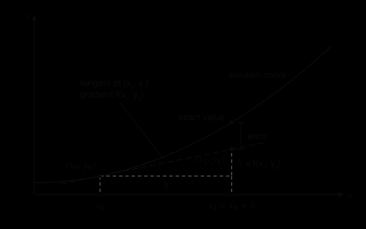
The method then repeats. At $(x_1, y_1)$ the differential equation gives a new gradient $f(x_1, y_1)$

The step length

The fixed horizontal distance $h$ moved in each step is the step length. It is chosen before the calculation starts and stays the same throughout.

To reach a target value $x = b$ from $x = x_0$, the number of steps is

For example, from $t = 0$ to $t = 1$ with $h = 0.25$ takes $\frac{1}{0.25} = 4$

The Euler formulas

Recurrence relations

Writing the step for a general point gives a pair of formulas that produce each new point from the one before. A formula of this kind is a recurrence relation, the same kind of rule that defines an arithmetic or geometric sequence term by term (subtopics 1.2 and 1.3).

The second formula says that $x$ goes up by the same amount every time: the values of $x$ form an arithmetic sequence with common difference $h$, so $x_n = x_0 + nh$

Carrying out the method by hand

On a short calculation, a table with one row per step keeps the working clear. The columns are $n$, $x_n$, $y_n$ and the gradient $f(x_n, y_n)$

Using technology

A real Euler calculation has tens or hundreds of steps, so it is always done with technology. Two approaches are common: a spreadsheet, which shows every value in a table, and the sequence mode of a GDC, which treats the Euler formulas as recurrence relations.

A spreadsheet set-up

A spreadsheet suits Euler's method because each row depends only on the row above it. With $h$ in a cell of its own, the method needs one row of starting values and one row of formulas, which is then filled down.

Spreadsheet for $\frac{\mathrm{d}y}{\mathrm{d}x} = x + y$, $y(0) = 1$

The dollar signs fix the reference to $h$, so changing the single value in B1 recalculates the whole table. This makes it easy to compare step lengths, which is the main way of judging accuracy.

The GDC's sequence mode

The sequence (recursion) mode of a GDC generates a sequence from a recurrence relation and lists the terms in a table. For Euler's method the sequence is $y_0, y_1, y_2, \ldots$, and the index $n$

The one complication is that $x$ usually appears in $f(x, y)$, but the sequence mode has no separate $x$ column. Since $x_n = x_0 + nh$

so every $x$ in the gradient is replaced by this expression.

1. Switch the GDC to sequence (recursion) mode (on a TI-84 Plus CE: MODE → SEQ; on a Casio fx-CG50: MENU → Recursion).

2. Enter the recurrence. For $\frac{\mathrm{d}y}{\mathrm{d}x} = x + y$ with $h = 0.1$

The row number $n$ is the number of steps, so the estimate of $y(b)$ is in the row $n = \frac{b - x_0}{h}$

What to write down

The table that technology produces is not itself the working. A clear Euler answer contains:

• the recurrence relations with the numbers substituted, for example $y_{n+1} = y_n + 0.5\big(0.5 - 0.05t_n - 0.15\sqrt{H_n}\big)$

YouTube

Step length and accuracy

Where the error comes from

Each Euler step assumes the gradient stays fixed at its starting value for the whole step. On a curved solution it does not, so every step lands slightly off the curve. Worse, the next step starts from that slightly wrong point, uses the gradient there, and adds its own error. Errors are carried forward and build up over the whole calculation.

The Euler polygon for $\frac{\mathrm{d}y}{\mathrm{d}x} = x + y$, $y(0) = 1$

Smaller steps, smaller errors

Halving the step length makes each segment shorter, so the gradient has less distance over which to go out of date. Repeating the calculation for $\frac{\mathrm{d}y}{\mathrm{d}x} = x + y$, $y(0) = 1$

Each time the step length is halved, the error roughly halves too. This pattern, error approximately proportional to $h$, holds for Euler's method in general when $h$ is small. Ten times the accuracy therefore needs about ten times as many steps. More advanced methods (the Runge–Kutta family) use several gradients per step to get much smaller errors for the same work.

A step length that is too large can give meaningless results. For the cooling equation $\frac{\mathrm{d}T}{\mathrm{d}t} = -0.15(T - 21)$ with $T(0) = 85$

Overestimate or underestimate

The direction of the error depends on which way the solution curve bends, its concavity. A tangent to a curve that is concave up lies below the curve, so following it gives values that are too small. A tangent to a curve that is concave down lies above it, so Euler's method gives values that are too large.

The direction of Euler's error over an interval on which the concavity does not change.

The concavity can be found without solving the equation. Differentiating $\frac{\mathrm{d}y}{\mathrm{d}x} = f(x, y)$ once more gives the second derivative. For $\frac{\mathrm{d}y}{\mathrm{d}x} = x + y$

which is positive whenever $x$ and $y$ are positive. The solution is concave up there, so Euler's method underestimates, as the example and the graph both showed. If the concavity changes within the interval (at a point of inflexion), the errors before and after partly cancel and the direction cannot be predicted this simply.

Comparing with an exact solution

When the equation can also be solved exactly by separation of variables, the comparison measures the accuracy of Euler's method directly. The percentage error is calculated in the usual way (subtopic 1.6), with the exact value as the reference. Comparisons of this kind show the general behaviour: the error grows with the number of steps taken and with the curvature of the solution, and shrinks roughly in proportion to $h$.

When no exact solution exists, the same check is made by repeating the calculation with half the step length. If the two estimates agree to the accuracy required, the step length is small enough; if they differ noticeably, the step length is halved again.

Euler's method for coupled systems

Coupled differential equations

Many systems involve two quantities that change together, each affecting the other's rate of change: a predator and its prey, two species competing for food, the numbers of healthy and infected people in an epidemic. Each quantity has its own differential equation, but each equation contains both variables.

The independent variable is now time $t$, and both $x$ and $y$ depend on it. Neither equation can be solved alone, because the rate for $x$ cannot be calculated without knowing $y$, and vice versa. Exact solutions exist only for special cases (linear systems, in subtopic 5.17, Phase portraits), so numerical solutions are the standard tool.

The coupled Euler formulas

Euler's idea carries over directly. At the current time $t_n$, both rates are known from the current values $x_n$ and $y_n$

Both new values are calculated from the old values $x_n$, $y_n$ and $t_n$

When the rates contain $t$ explicitly (a seasonal birth rate, a harvest that increases each year), the time column matters: $t_n$ must be updated each step and used in both rates. When they do not, as in most population models, $t$ still counts the steps and shows when each value occurs.

Technology for coupled systems

On a spreadsheet, a coupled system needs one column for each variable and one for time. Each formula in a new row refers only to cells in the row above, which builds the simultaneous update into the layout.

Spreadsheet for the deer–wolf model with h = 0.1: row 3 is filled down; every formula in row 3 refers to row 2 only.

In GDC sequence mode, the two variables become two sequences, $u(n)$ for $x$ and $v(n)$ for $y$, each defined from both $u(n-1)$

• $u(n) = u(n-1) + 0.1\big(0.5u(n-1) - 0.01u(n-1)v(n-1)\big)$

The table then lists both sequences side by side, with $n$ as the step number and $t = 0.1n$. Because both formulas use the previous terms, the calculator performs the simultaneous update correctly. A calculator using the $a_{n+1}$, $b_{n+1}$

Predator–prey models

The Lotka–Volterra equations

The deer–wolf system is an example of the best-known coupled model in biology. Prey (deer) grow when left alone; predators (wolves) die out when left alone; and every meeting between the two helps the predators and harms the prey.

Each term has a meaning, and reading the terms is a common first step in any question about such a model.

The four terms of a predator–prey model and what each represents.

The product $xy$ appears in both equations because the number of encounters between predators and prey depends on how many of each there are: doubling either population doubles the encounters. The constants $b$ and $c$ differ because one kill removes one prey but produces only a fraction of a new predator.

Equilibrium points

An equilibrium point is a state in which nothing changes: both rates are zero at once. For a predator–prey model,

Both rates are zero at $(0, 0)$, where both species are absent, and at $\left(\frac{d}{c}, \frac{a}{b}\right)$

The equilibrium values also explain the turning points of the populations. The prey stop increasing and start decreasing exactly when $y$ passes $\frac{a}{b}$, and the predators turn exactly when $x$ passes $\frac{d}{c}$

Trajectories in the phase plane

Running the deer–wolf model with $h = 0.1$ for 20 years produces 200 rows of values. Plotting $y$ against $x$ from these rows, instead of each against $t$, gives a path in the phase plane called a trajectory. The trajectory of the deer–wolf model from $(400, 40)$

Following the loop round shows the four stages of the cycle. With few wolves, deer increase (moving right). Plenty of deer lets wolves increase (moving up). Many wolves cut the deer population (moving left), and with fewer deer the wolves decline (moving down), returning to the start. From the full table, the deer reach a maximum of about 738 at $t \approx 6.9$, when $y \approx 50$, and the wolves a maximum of about 65 at $t \approx 11.2$, when $x \approx 500$

The exact solutions of the Lotka–Volterra equations are closed loops that repeat for ever. The Euler trajectory does not quite close: after 20 years it reaches $(386, 39)$ instead of $(400, 40)$, and further cycles drift slowly outwards. The exact model has no such drift, so it comes from accumulated error; repeating the run with $h = 0.01$ makes the loop very nearly close.

Competing species models

Two species, one food supply

Two species that eat the same food do not prey on each other, but each one's presence slows the other's growth. Each species alone would follow a logistic model, levelling off at its carrying capacity; the competition adds a term that reduces each growth rate in proportion to the other population.

A typical form is

The bracket in each equation shows the room left to grow. Without $y$, the first species levels off at $x = A$; each animal of the second species uses up the resources of $p$ animals of the first. The constants $p$ and $q$ measure how strongly each species competes.

Setting both rates to zero gives up to four equilibrium points: $(0, 0)$, $(A, 0)$, $(0, B)$, and a point where both species survive, found by solving the two linear equations $x + py = A$

Long-term behaviour from further iterations

Whether the species coexist or one drives the other out depends on the constants and, sometimes, on the starting numbers. Euler's method answers the question numerically: run the recurrences for many steps and watch where the values settle.

With stronger competition the outcome changes. If each species harms the other more than it harms itself, the coexistence point becomes unstable, and the species that starts with the advantage wins while the other dies out. Different starting values can then lead to different long-term outcomes, which is the behaviour of a saddle point in subtopic 5.17.

The SIR model of an epidemic

Three groups of people

The SIR model divides a population of size $N$ into people who can catch a disease (susceptible, $S$), people who have it and can pass it on (infected, $I$), and people who have recovered and are immune (recovered, $R$). Kermack and McKendrick introduced it in 1927, and models built on it are still used to plan for epidemics.

The term $\frac{\beta SI}{N}$ counts new infections: it grows with the number of infected people spreading the disease and with the proportion $\frac{S}{N}$

Euler's method with a step of one day

With $N = 1000$, $\beta = 0.5$ per day, $\gamma = 0.25$ per day (people stay infected for 4 days on average), and 10 infected people at the start, Euler's method with $h = 1$

The first step gives $S_1 = 990 - 4.95 = 985.05$ and $I_1 = 10 + 4.95 - 2.5 = 12.45$

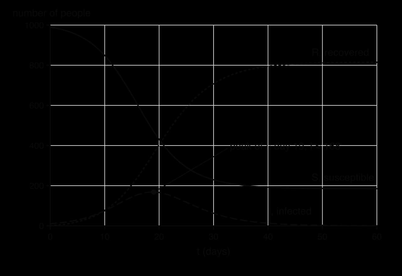
The peak can be predicted without the table. The number infected stops rising when $\frac{\mathrm{d}I}{\mathrm{d}t} = 0$:

Infections rise while more than 500 people are susceptible and fall once fewer are. In the Euler table, $S$ passes 500 between day 18 (513) and day 19 (470), and $I$ is greatest on day 19, at about 168. The epidemic dies out while about 185 people are still susceptible: by then there are too few of them for each infected person to pass the disease to more than one other.

YouTube

Euler's method in reverse: estimating a rate from data

The Euler step can also be read backwards. If a quantity $N$ satisfies $\frac{\mathrm{d}N}{\mathrm{d}t} = rN$ and values are recorded at intervals of 1 unit of time, one Euler step with $h = 1$

Each pair of consecutive data values then gives an estimate of the growth constant $r$: the change over one interval divided by the value at the start of the interval. This turns a table of data into estimates of a parameter in a differential equation.

Case study: Hudson's Bay Company lynx and hare pelts

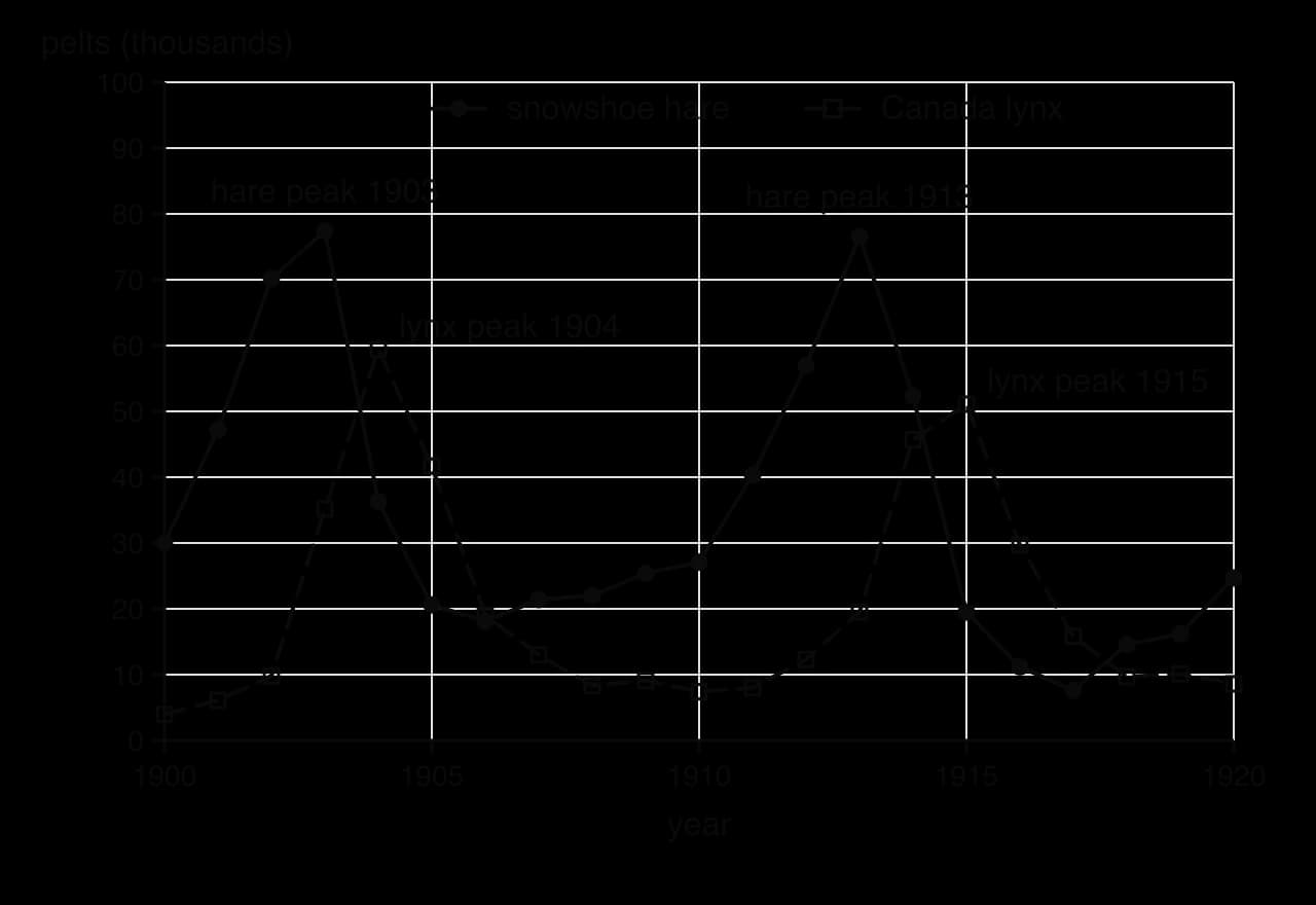
For much of its history, the Hudson's Bay Company bought furs from trappers across Canada, and its records of the numbers of pelts traded each year are one of the best-known long-term population records in ecology. The pelts of the snowshoe hare and of its main predator, the Canada lynx, rise and fall in a cycle of about ten years, with the lynx peaks following the hare peaks.

Source: Hudson's Bay Company pelt records, 1900–1920, as tabulated in B. Carpenter, “Predator–Prey Population Dynamics: the Lotka–Volterra model in Stan”, Stan case study, 2018.

The full record for 1900–1920 shows two complete cycles. Each lynx peak comes one or two years after a hare peak, the kind of lag that the predator–prey model predicts.

Fitting the model

Fitting the predator–prey model to the 1900–1920 data, with hares $H$ and lynx $L$ in thousands and $t$ in years, gives parameter estimates of about $a = 0.55$, $b = 0.028$, $c = 0.024$

The non-zero equilibrium is $H = \frac{0.80}{0.024} = 33.3$ and $L = \frac{0.55}{0.028} = 19.6$

Running Euler's method from 1900

Starting from the 1900 values $H_0 = 30.0$, $L_0 = 4.0$, the recurrences with $h = 0.1$

The first step gives $H_1 = 30 + 0.1(16.5 - 3.36) = 31.314$ and $L_1 = 4 + 0.1(2.88 - 3.2) = 3.968$

Euler estimates (thousands of pelts) from the fitted model, starting from the 1900 data; calculated values.

Interpreting the results

The model reproduces the main features of the first cycle: the hare peak in 1903, the lynx peak about a year later, and the collapse of both. It is less successful in the details: the modelled lynx numbers rise too slowly before the peak (22.3 thousand in 1903 against 35.2 in the data), and the modelled hares fall to about 9 thousand in 1907, well below the observed minimum of 18.1 thousand in 1906. The step length matters too. The two runs agree in the first two years but differ by more than 6 thousand hares in 1904, and with $h = 0.1$ the lynx peak even moves a year late, to 1905. Run further, the $h = 0.1$ solution grows a little with each cycle (a hare peak of about 101 thousand in 1914), the same outward drift seen in the deer–wolf trajectory, while the $h = 0.01$ run keeps a nearly steady cycle.

The comparison also shows the limits of the model itself. Pelt counts measure the number of animals trapped, which depends on trapping effort and fur prices as well as on population size. The hare cycle is also affected by food supply and by other predators, which the two-species model leaves out, and the model is deterministic, while real populations vary randomly from year to year. A model that captures the period and the lag but not the exact sizes of the peaks is useful for explaining why the cycle exists, but not for forecasting a particular year's numbers.

Exam focus

Euler's method appears on Paper 2 and Paper 3, usually as 3–6 marks inside a long modelling question that also uses separation of variables (subtopic 5.14), equilibrium points or phase portraits (5.17), or a model fitted to data. Questions use Euler's method with a given step length to find or estimate values, ask you to write down the recurrence relations, to sketch a trajectory from Euler values, and to comment on accuracy or explain the meaning of terms in a model. The values are always produced with the GDC; what earns the method marks is the recurrence relations written with the numbers substituted.

Common question shapes:

• a single equation $\frac{\mathrm{d}y}{\mathrm{d}x} = f(x, y)$, with a comparison against an exact solution found earlier in the question;

• a predator–prey or competing species system: interpret the terms, find the equilibrium points by setting both rates to zero, run Euler to a given time, then use further iterations for the long-term behaviour;

• a sketch of the trajectory in the phase plane from an Euler table;

• a reason why a result might be unreliable (step length too large, estimated parameters, factors left out of the model).

Examiners consistently reward the recurrence relations. A table of values with a wrong final answer and no formulas can score nothing, while correct formulas with an arithmetic slip still earn the method marks. Write the formulas with the actual numbers substituted, not the general booklet form.

YouTube

Practice questions

1. The function $y$ satisfies $\frac{\mathrm{d}y}{\mathrm{d}x} = 2x - y$, and $y = 3$

2. The function $y$ satisfies $\frac{\mathrm{d}y}{\mathrm{d}t} = t^2 - 0.5y$

3. A population of birds on an island, $P$, is modelled by $\frac{\mathrm{d}P}{\mathrm{d}t} = 0.04P\left(1 - \frac{P}{500}\right)$

4. The function $y$ satisfies $\frac{\mathrm{d}y}{\mathrm{d}x} = 3 - 0.5y$, with $y = 0$

5. The numbers of prey, $x$, and predators, $y$, in a nature reserve are modelled by $\frac{\mathrm{d}x}{\mathrm{d}t} = x(1 - 0.05y)$

6. Two competing species have populations $x$ and $y$ (in thousands) modelled by $\frac{\mathrm{d}x}{\mathrm{d}t} = x(4 - x - 2y)$

7. In a town of 500 people, an infection is modelled by $\frac{\mathrm{d}S}{\mathrm{d}t} = -\frac{0.4SI}{500}$

8. The number of subscribers to a new podcast at the start of four consecutive months is 1200, 1380, 1590 and 1820. The growth is modelled by $\frac{\mathrm{d}N}{\mathrm{d}t} = rN$, with $t$ in months. (a) Show that Euler's method with step length 1 gives $r \approx \frac{N_{n+1} - N_n}{N_n}$

Summary

• Euler's method follows the tangent for a short step: $y_{n+1} = y_n + h \times f(x_n, y_n)$

Self-check

• To do:

  I can explain why one Euler step moves along the tangent and what the rise $h \times f(x_n, y_n)$ represents.

• To do:

  I can calculate the number of steps needed to reach a given value.

• To do:

  I can carry out two or three Euler steps by hand in a table.

• To do: