5.17 Phase portraits

Learning objectives

• Write down a system of coupled linear differential equations $\dot{x} = ax + by$, $\dot{y} = cx + dy$ in the matrix form $\dot{\boldsymbol{x}} = M\boldsymbol{x}$.

• Find the equilibrium points of a system of coupled differential equations, linear or non-linear.

• Find the gradient $\frac{\mathrm{d}y}{\mathrm{d}x}$ of a trajectory at a point in the phase plane.

• Find the general solution $\boldsymbol{x} = A\mathrm{e}^{\lambda_1 t}\boldsymbol{p}_1 + B\mathrm{e}^{\lambda_2 t}\boldsymbol{p}_2$

• Determine the type and stability of the equilibrium point at the origin from the eigenvalues: real, complex or purely imaginary.

• Sketch a phase portrait or a single trajectory, showing eigenvector lines, asymptotic behaviour and the direction of motion.

• Interpret a phase portrait in context: which populations survive, which quantity dies out, and what happens in the long term.

Introduction

Many real systems contain two quantities that change together and affect each other: two species sharing a forest, a medicine moving between the blood and the body's tissues, the charge and current in a circuit. Each rate of change depends on both quantities, so the two differential equations cannot be solved one at a time. When the dependence is linear, the whole system is described by a single 2 × 2 matrix, and the eigenvalues and eigenvectors of that matrix give its exact solution and its long-term behaviour.

A phase portrait shows that behaviour as a picture. Instead of drawing each quantity against time, it plots one quantity against the other, so that every solution becomes a path in the plane. A glance at the portrait shows whether the system settles down, grows without limit, spirals or cycles, and which starting values lead to which outcome.

Coupled linear systems in matrix form

Two rates that depend on each other

Subtopic 5.16, Euler's method, introduced coupled differential equations, pairs of equations in which the rate of change of each variable depends on both variables. In dot notation, $\dot{x}$ means $\frac{\mathrm{d}x}{\mathrm{d}t}$ and $\dot{y}$

The right-hand sides have exactly the shape of a matrix multiplying a column vector. Writing $\boldsymbol{x} = \begin{pmatrix} x \\ y \end{pmatrix}$ and $\dot{\boldsymbol{x}} = \begin{pmatrix} \dot{x} \\ \dot{y} \end{pmatrix}$

The first row of $M$ holds the coefficients of the $\dot{x}$ equation and the second row those of the $\dot{y}$ equation. Within each row, the first column multiplies $x$ and the second multiplies $y$

Reading a model term by term

Each entry of $M$ has a meaning in context. In a model of two species, the diagonal entries $a$ and $d$ describe how each population changes on its own (a positive value means natural growth, a negative value means decline), and the off-diagonal entries $b$ and $c$ describe how each species affects the other.

The same reading works outside ecology. In a model of a medicine, $x$ and $y$ can be the amounts in the blood and in the tissues: a negative diagonal entry is the rate at which the medicine leaves a compartment, and a positive off-diagonal entry is the rate at which it arrives from the other one.

The phase plane and trajectories

Two ways to draw one solution

A solution of a coupled system is a pair of functions $x(t)$ and $y(t)$. One way to show it is a pair of time series: $x$ against $t$ and $y$ against $t$

The second way removes time from the axes. Each instant $t$ gives a point $(x(t), y(t))$, and as $t$ increases the point moves and traces a curve. The plane in which this curve is drawn is the phase plane.

The curve that one solution traces is its trajectory. Time is still present, but only as the position along the curve and the direction of motion, which is shown with arrows.

Time series and trajectories carry the same information, organised differently. The time series shows when things happen (the tissue peak at 0.462 hours); the trajectory shows how the two quantities relate (the tissue amount is greatest when the trajectory reaches its highest point, and in the long run the tissue holds twice as much medicine as the blood). A trajectory is drawn with $y$ against $x$, never against $t$.

Phase portraits

Drawing one trajectory shows the future from one starting point. Drawing several, from starting points spread around the plane, shows the behaviour of the whole system.

Two facts make a phase portrait readable. First, through each point of the plane there passes exactly one trajectory, because the equations fix the direction of motion at every point; so trajectories never cross. Second, for an autonomous system (one in which $t$ does not appear on the right-hand side), the trajectory through a point does not depend on when the system arrives there, so the portrait is the same picture for all time.

Equilibrium points

Where both rates are zero

A point where $\dot{x} = 0$ and $\dot{y} = 0$ at the same time is special, because a system that starts there does not move and stays there for ever.

For a linear system $\dot{\boldsymbol{x}} = M\boldsymbol{x}$, equilibrium needs $M\boldsymbol{x} = \boldsymbol{0}$. The origin always satisfies this. If $\det M \neq 0$

A trajectory never reaches an equilibrium point in a finite time: it can only approach it as $t \to \infty$ (or leave it as $t \to -\infty$). This follows from the "no crossing" rule, because the equilibrium point is itself a trajectory consisting of a single point.

Equilibrium points of non-linear systems

The method extends to the non-linear models of subtopic 5.16, such as the predator–prey model and the competing species model: set both rates equal to zero and solve the two equations simultaneously. A product such as $x(4 - x - y)$ is zero when either factor is zero, so each equation usually gives two cases, and every combination must be checked.

Whether a non-linear system actually settles at one of its equilibria depends on the behaviour of trajectories near each point, which is found by linearising the system there with a matrix of partial derivatives called the Jacobian. That analysis is an extension; for linear systems the eigenvalues of $M$ give the answer directly.

The gradient of a trajectory

Dividing one rate by the other

Along a trajectory, $y$ can be treated as a function of $x$ (at least locally), and the chain rule gives $\frac{\mathrm{d}y}{\mathrm{d}t} = \frac{\mathrm{d}y}{\mathrm{d}x} \times \frac{\mathrm{d}x}{\mathrm{d}t}$

The gradient is the direction of motion at that point, so it is exactly the information a slope field displays. Two special cases help with sketching:

• where $\dot{y} = 0$ (but $\dot{x} \neq 0$), the trajectory is horizontal;

• where $\dot{x} = 0$

These lines are the nullclines of the system. The gradient alone does not give the direction of travel along the curve: the sign of $\dot{x}$ shows whether the point moves right ($\dot{x} > 0$) or left ($\dot{x} < 0$

Exact solutions for real distinct eigenvalues

Why eigenvectors give solutions

For a single equation $\dot{x} = kx$, subtopic 5.14 showed the solution is $x = A\mathrm{e}^{kt}$. This suggests looking for solutions of $\dot{\boldsymbol{x}} = M\boldsymbol{x}$

These are equal for all $t$ exactly when $M\boldsymbol{p} = \lambda\boldsymbol{p}$, that is, when $\boldsymbol{p}$ is an eigenvector of $M$ and $\lambda$ its eigenvalue. So each eigenvalue–eigenvector pair gives a solution that moves along a straight line through the origin, outwards if

The system is linear, so the sum of two solutions is also a solution (differentiation and matrix multiplication both distribute over addition), and so is any constant multiple. With two real distinct eigenvalues $\lambda_1, \lambda_2$ and eigenvectors $\boldsymbol{p}_1, \boldsymbol{p}_2$

This is the general solution. The two arbitrary constants $A$ and $B$ match the two pieces of information needed to fix a solution: the starting values $x(0)$ and $y(0)$. At $t = 0$ both exponentials equal 1, so the initial vector is

The method

The eigenvalues come from the characteristic equation $\det(M - \lambda I) = 0$ of subtopic 1.15. For a 2 × 2 matrix it is a quadratic in terms of the trace and the determinant:

1. Write the system as $\dot{\boldsymbol{x}} = M\boldsymbol{x}$.

2. Solve $\lambda^2 - (\operatorname{tr} M)\lambda + \det M = 0$

On the GDC, the characteristic equation is solved with the polynomial root finder (on a TI-84 Plus CE: APPS → PlySmlt2 → POLYNOMIAL ROOT FINDER; on a Casio fx-CG50: MENU → Equation → POLY). The TI-Nspire can return the eigenvalues and eigenvectors of a matrix directly, but its Press-to-Test mode blocks these functions, so the characteristic equation method is the one to know. Either way, write down the characteristic equation and the eigenvalues, and show the equation used for each eigenvector.

YouTube

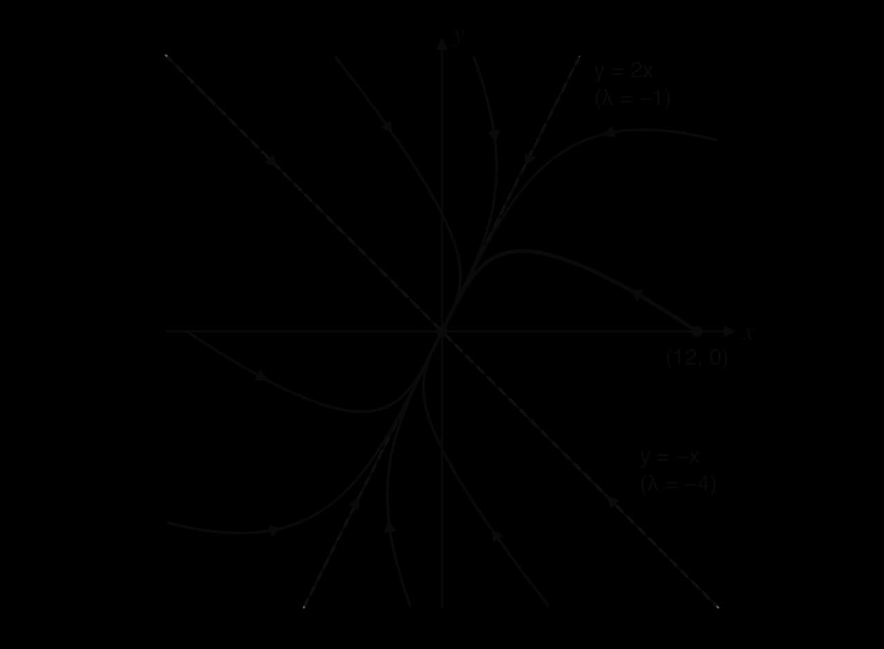
The phase portrait of the medicine model shows what part (e) means geometrically. The two eigenvector lines, $y = 2x$ and $y = -x$, are straight-line trajectories. Every other trajectory, including the bold one from $(12, 0)$, curves round and enters the origin along $y = 2x$

Long-term direction and the dominant eigenvalue

Writing the solution with the larger eigenvalue first shows which term controls the long run. Suppose $\lambda_1 > \lambda_2$ and $A \neq 0$. Then

and since $\lambda_2 - \lambda_1 < 0$, the second term inside the bracket tends to 0 as $t \to \infty$. The direction of $\boldsymbol{x}$

• As $t \to \infty$, trajectories line up with the eigenvector of the larger eigenvalue (the one further right on the number line).

• As $t \to -\infty$, they line up with the eigenvector of the smaller eigenvalue.

For the medicine model, $-1 > -4$, so trajectories approach the origin along $\begin{pmatrix} 1 \\ 2 \end{pmatrix}$. The exception is a trajectory with $A = 0$

Classifying the equilibrium point

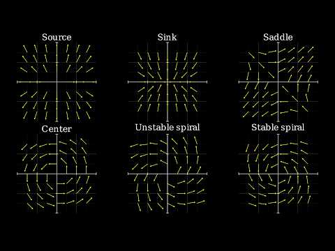
The eigenvalues decide the shape of the whole portrait. Each case has a name, a typical picture and a stability description. The ideas of stable and unstable equilibrium apply to all of them.

A stable equilibrium describes a system that recovers from small disturbances: medicine cleared from the body, a pollutant flushed from a lake, a car body settling after a bump. Its opposite describes a system that runs away from the balance point.

Real eigenvalues with the same sign: nodes

When both eigenvalues are real and have the same sign, every solution is a sum of two exponentials that both decay or both grow. Trajectories are straight along the eigenvector lines and gently curved elsewhere, with no turning round the origin.

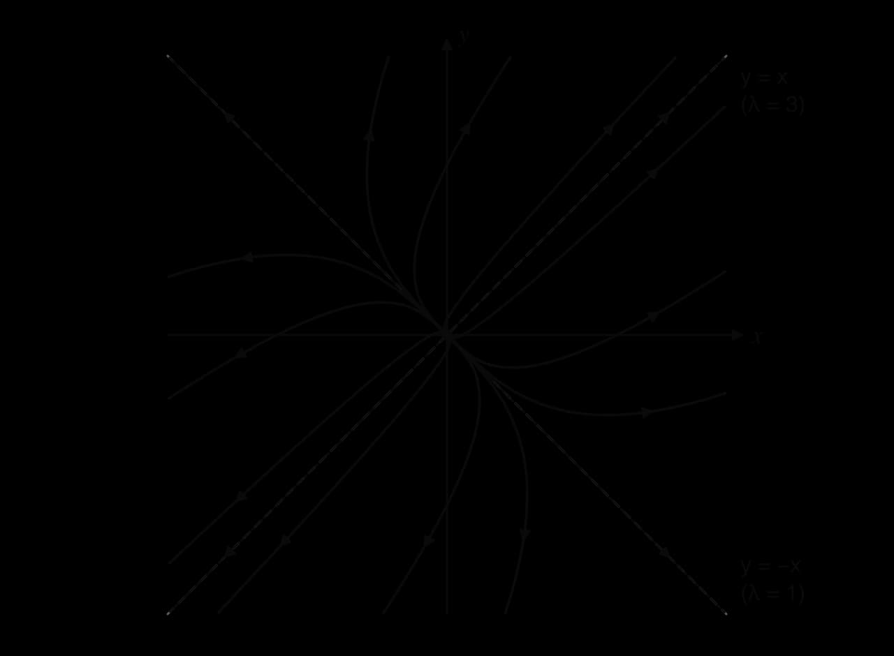
The medicine model is a stable node. When both eigenvalues are positive, every arrow is reversed and the origin is an unstable node. Near the origin, trajectories leave tangent to the eigenvector of the smaller eigenvalue (it dominates as $t \to -\infty$); far from the origin they run parallel to the eigenvector of the larger eigenvalue.

Real eigenvalues with opposite signs: saddle points

When one eigenvalue is positive and the other negative, the solution has one decaying term and one growing term. A trajectory that starts exactly on the eigenvector line of the negative eigenvalue moves straight into the origin. Every other trajectory approaches for a while, then is carried away along the eigenvector line of the positive eigenvalue.

The name comes from the shape of a horse's saddle, which slopes down towards its centre in one direction and away from it in the other. A saddle point is always unstable, because almost every starting point eventually leads away from it. The incoming eigenvector line separates the starting points that end up going one way from those that go the other way.

Case study: competing squirrels

Grey squirrels were introduced to Britain from North America in the 1870s. Competing with the native red squirrel for food, and carrying a disease that is often fatal to red squirrels, they have replaced it across most of England and Wales; most of the red squirrels left in the UK now live in Scotland. A simple linear competition model shows how one species can push out another.

Suppose that the numbers of red squirrels $x$ and grey squirrels $y$ in a woodland (in hundreds) follow the hypothetical model

with $t$ in years. The negative off-diagonal entries show competition. The trace is $0.4$ and the determinant is $0.03 - 0.08 = -0.05$, so

For $\lambda = 0.5$: $-0.2p - 0.4q = 0$, eigenvector $\begin{pmatrix} 2 \\ -1 \end{pmatrix}$

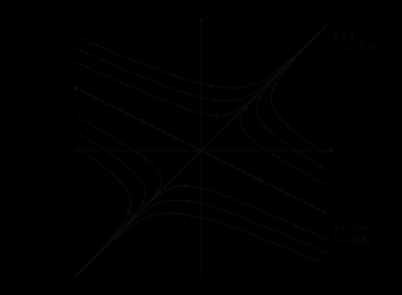
The general solution is

From $x(0) = x_0$ and $y(0) = y_0$: $2A + B = x_0$

• If $x_0 > y_0$, then $A > 0$: the growing term pushes the point in the direction $(2, -1)$

With $x_0 = 5$ and $y_0 = 4$ (500 red and 400 grey squirrels), $A = \frac{1}{3}$

Setting $y = 0$ gives $\mathrm{e}^{0.6t} = 13$, so $t = \frac{\ln 13}{0.6} = 4.27$

The model shows the qualitative point clearly. When the competition terms are strong compared with each species' own growth rate, the two populations cannot settle together, and a small initial advantage decides which species takes over. The model also has clear limitations. A linear model lets the winner grow without limit, ignores the disease that has done much of the harm to red squirrels, and stops making sense once a population reaches zero. Real conservation work, such as removing grey squirrels to protect red ones on the island of Anglesey in Wales since 1998, changes the starting point so that it lies on the "red" side of the dividing line.

Sources: Wikipedia, "Red squirrel" and "Eastern gray squirrel", accessed 2026. Model coefficients are hypothetical.

Complex eigenvalues: spirals

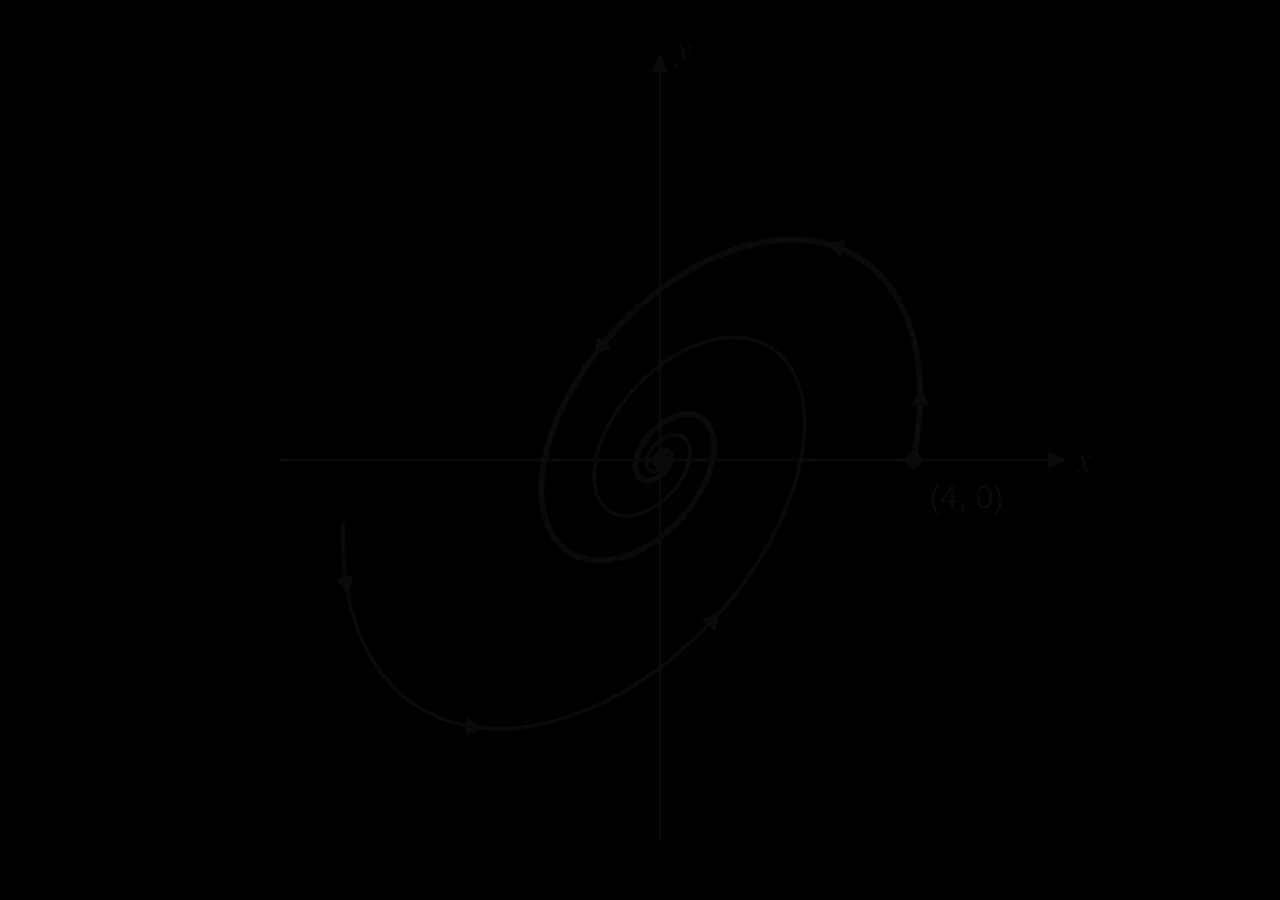
When the characteristic equation has a negative discriminant, the eigenvalues are a conjugate pair of complex numbers $\lambda = \alpha \pm \beta\mathrm{i}$. There are no real eigenvectors, so no trajectory is a straight line through the origin. Instead the solutions combine a factor $\mathrm{e}^{\alpha t}$, which sets the size, with sine and cosine terms in $\beta t$

• If $\alpha < 0$, the size shrinks while the point turns: trajectories spiral into the origin.

• If $\alpha > 0$, the size grows: trajectories spiral outwards.

Clockwise or anticlockwise

The eigenvalues do not show the direction of turning. It comes from the equations themselves: on the positive $x$-axis, $y = 0$, so $\dot{y} = cx$.

• If $c > 0$, $\dot{y} > 0$ on the positive $x$-axis: the point moves upwards there, so the motion is anticlockwise.

• If $c < 0$

The same check works on the positive $y$-axis, where $\dot{x} = by$: $b > 0$ means moving right, which is clockwise. For complex eigenvalues $b$ and $c$

The rate at which a spiral shrinks comes from the real part and the speed of turning from the imaginary part. One full turn takes time $\frac{2\pi}{\beta}$, during which the size changes by a factor of $\mathrm{e}^{2\pi\alpha/\beta}$. For the system in the worked example, one turn takes $\frac{2\pi}{2} = \pi \approx 3.14$

Purely imaginary eigenvalues: centres

If the real part is zero, the eigenvalues are purely imaginary, $\pm\beta\mathrm{i}$. The size neither grows nor shrinks, so each trajectory returns to its starting point and goes round the same closed curve for ever. For a linear system these curves are ellipses (circles in special cases) centred on the origin. Purely imaginary eigenvalues occur exactly when the trace $a + d$ is zero and the determinant is positive.

A centre is neither an attractor nor a repeller: a solution that starts near it stays near it for ever but never reaches it. Some texts call this "neutrally stable"; it is not a stable equilibrium in the sense used for nodes and spirals, because nearby trajectories do not approach it.

A memorable centre comes from a light-hearted model of love by the mathematician Steven Strogatz. Romeo's love for Juliet is $R$ and Juliet's love for Romeo is $J$ (negative values mean dislike). Juliet's love grows when Romeo loves her, but Romeo is contrary: the more Juliet loves him, the faster his love falls. With hypothetical constants,

The matrix $\begin{pmatrix} 0 & -1 \\ 4 & 0 \end{pmatrix}$ has trace 0 and determinant 4, so $\lambda^2 + 4 = 0$

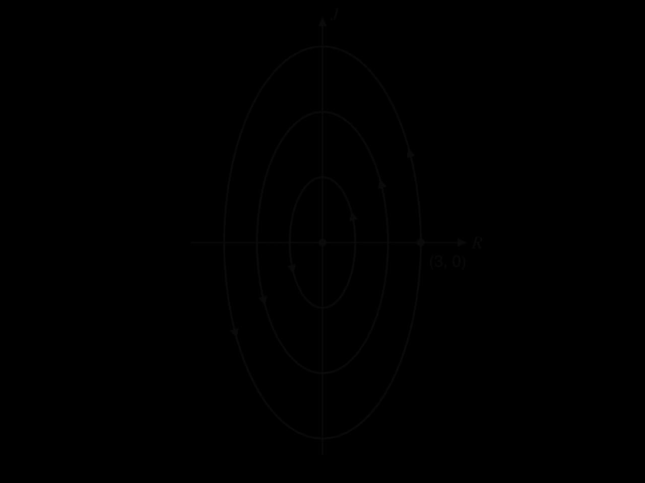
Starting from $(3, 0)$, Romeo loves Juliet and she is indifferent. Her love then grows, which makes his fall; he becomes indifferent, then hostile, which makes her love fall, and so on round the ellipse. One cycle takes $\frac{2\pi}{2} = \pi$ time units. The ellipses satisfy $4R^2 + J^2 = \text{constant}$

Predator–prey populations such as the snowshoe hare and lynx records of subtopic 5.16 also go round closed loops in the phase plane, but their model is non-linear, so the loops are not ellipses.

Summary of the classification

YouTube

Sketching phase portraits

What every sketch shows

A phase portrait is a sketch, not an accurate plot, but it must show the features that the eigenvalues predict. The following checklist covers all the cases.

1. Axes labelled with the two variables ($x$ and $y$, or the names in the question), with the equilibrium point at the origin.

2. Eigenvector lines (real eigenvalues only), drawn as straight lines through the origin, with arrows inwards for a negative eigenvalue and outwards for a positive one.

3. At least three trajectories that do not cross each other or the eigenvector lines, shaped by the dominant eigenvector rules (nodes and saddles) or winding the correct way (spirals and centres).

4. Arrows on every trajectory showing the direction of motion as $t$ increases.

5. Any point or gradient the question asks for, for example a trajectory starting at a given point with a gradient found from $\frac{\dot{y}}{\dot{x}}$

When only one trajectory is required, start at the given point, set off with the correct gradient and direction (from $\dot{x}$ and $\dot{y}$ at that point), and finish by approaching the correct eigenvector direction.

Exam focus

Phase portraits and coupled systems are examined on HL Paper 1 (4–6 marks: a gradient and a sketch, or a classification), Paper 2 (10–18 marks: a full modelling question) and Paper 3 (an investigation that may build the method from earlier parts). Questions are almost always set in context: competing or symbiotic species, fungi or moss on a tree, pollution in lakes or rivers. The eigenvalue and eigenvector parts follow the method of subtopic 1.15 and earn the same marks.

The recurring shapes and command terms are:

• find the eigenvalues and eigenvectors: (M1) for $\det(M - \lambda I) = 0$, (A1) for the characteristic equation, A1 for the values; (M1) for an attempt at an eigenvector, A1 each, any non-zero multiple accepted;

• hence write down the general solution: (M1)A1, with the left-hand side $\begin{pmatrix} x \\ y \end{pmatrix}$

Part (g) is where most marks are lost. The trajectory starts at $(6, 1)$ with $\dot{x} < 0$ and $\dot{y} > 0$

When the question gives the eigenvalues and eigenvectors, use them straight away; a sketch question may hinge only on knowing which eigenvector the trajectory approaches. When the question asks for "$x$ in terms of $t$", finish with $x = \ldots$, not with the vector form. When the command term is state or write down, no working is expected: classifying from given eigenvalues is a one-line answer.

Practice questions

1. Write down the matrix $M$ for the system $\dot{x} = 3y - x$, $\dot{y} = 2x$

Summary

• A linear system $\dot{x} = ax + by$, $\dot{y} = cx + dy$

Self-check

• To do:

  I can write a coupled linear system as $\dot{\boldsymbol{x}} = M\boldsymbol{x}$, with every coefficient in the correct row and column.

• To do:

  I can interpret the signs of the entries of $M$ as growth, decline, competition, symbiosis or predation.

• To do:

  I can find all the equilibrium points of a linear or non-linear system.

• To do:

  I can explain the difference between a time-series graph and a trajectory in the phase plane.

• To do:

  I can find $\frac{\mathrm{d}y}{\mathrm{d}x}$