Augment Education
    • Question bank
    • Quick fire
    • Worksheets
    • Flashcards
    • Notes
    • Try a quick-fire round
    • All features
    • Business
    • Digital Society
    • Economics
    • Geography
    • Global Politics
    • History
    • Philosophy
    • Psychology
    • Anthropology
    • World Religions
    • Biology
    • Chemistry
    • Physics
    • Computer Science
    • Design Technology
    • ESS
    • SEHS
    • Language and literature
    • Language acquisition
    • Maths AA
    • Maths AI
    • Dance
    • Film
    • Music
    • Theatre
    • Visual Arts
    • Grade calculator
    • Grade boundaries
    • Subject checker
    • Focus timer
    • Exam countdown
    • All free tools
    • IB guide
    • All subjects
  • Blog

Search

Search subjects, the syllabus, glossary terms, the booklets, the IB guide, help and the blog

Log inStart free
augment

Augment Education

IB Diploma revision built around the syllabus.

contact@augment-education.com

Product

  • Features
  • Question bank
  • Quick fire
  • Worksheets
  • Flashcards
  • Notes
  • Subjects
  • What's new

Learn

  • IB guide
  • Booklets, explained
  • Glossary
  • Blog
  • Free tools
  • Grade calculator
  • Subject checker

Company

  • About
  • Help
  • For parents
  • For teachers
  • Comparisons

Subjects

  • English A Lit
  • English A Lang & Lit
  • Chinese A Lit
  • Chinese A Lang & Lit
  • Spanish A Lit
  • Spanish A Lang & Lit
  • English Lit & Perf
  • Spanish Lit & Perf
  • English B
  • Mandarin B
  • Spanish B
  • English ab initio
  • Mandarin ab initio
  • Spanish ab initio
  • Business
  • Digital Society
  • Economics
  • Geography
  • Global Politics
  • History
  • Philosophy
  • Psychology
  • Anthropology
  • World Religions
  • Biology
  • Chemistry
  • Physics
  • Computer Science
  • Design Technology
  • ESS
  • SEHS
  • Maths AA
  • Maths AI
  • Dance
  • Film
  • Music
  • Theatre
  • Visual Arts

Augment Education is developed independently of the International Baccalaureate Organization and is not endorsed by it. “IB” and “International Baccalaureate” are its trademarks.

© 2026 Augment Education. All rights reserved.

  • Privacy
  • Terms
  1. Subjects
  2. Geography
  3. Geographic skills: maps, graphs and data

Geographic skills: maps, graphs and data

Locate places with grid references and scale, read and construct every map and graph type the course uses, summarise data with simple calculations, describe patterns with figures and evaluate sources.

  • IB Geography
  • Exam skills
  • SL and HL

48 min readLast reviewed 18 Oct 2026

What geographic skills are

Geographic skills are the techniques geographers use to locate places, read and draw maps and graphs, summarise data with simple calculations and judge how far a source can be trusted. They are tools for thinking about place, process and pattern: a choropleth map shows where a variable is high or low, a cross-section shows the shape of a valley, and a mean or a percentage change turns a column of numbers into a statement that can be compared with another place.

Skills run through every part of the course. In Paper 1 the structured question on each option is built on a stimulus, often a topographic map extract, a graph or a table, and its first parts ask you to read values, grid references, directions and differences from it. In Paper 2, Section A questions open with a figure to describe, and Section B is built on an infographic. The fieldwork report depends on the same skills in reverse: there you collect the data, choose the graphs and maps, and draw them yourself.

Exam tip

Short skills questions are worth 1 or 2 marks each, but they are the most reliable marks on the paper. Read the figure exactly: give units (m, km, °C, %), the direction or grid reference in the form asked for, and figures read as accurately as the scale allows. An answer without a unit, or with "about" where a precise reading is possible, often loses the mark.

Locating places

Latitude and longitude

Any point on the Earth’s surface can be located by latitude and longitude. Latitude is the angle north or south of the Equator (0°), up to 90° N or 90° S at the poles; lines of latitude (parallels) run east–west. Longitude is the angle east or west of the Prime Meridian through Greenwich (0°), up to 180° E or W; lines of longitude (meridians) run north–south. Degrees are divided into 60 minutes, so 51° 30′ N is halfway between 51° N and 52° N.

A location is written latitude first: Nairobi lies at about 1° 17′ S, 36° 49′ E. Latitude matters in many explanations, because it controls the angle of the Sun and therefore temperature, and the position of the major pressure belts. On world maps in the exam you may be asked to state the latitude of a feature or to describe a distribution by latitude ("most tropical cyclones form between 5° and 20° north and south of the Equator").

Direction and bearings

Direction is given as one of the eight points of the compass (N, NE, E, SE, S, SW, W, NW), or of sixteen for more precision (NNE, ENE and so on). A bearing is more exact: the angle measured clockwise from north, written with three figures (045° is north-east, 270° is west). Directions are always given from one place to another: if a church is south-west of a hill, the hill is north-east of the church.

Tip

Describe the direction a river flows towards, not where it comes from: a river that flows from the north-west to the south-east "flows south-east". Winds are the opposite: a south-westerly wind blows from the south-west.

Scale and distance

A map scale is the ratio between a distance on the map and the same distance on the ground. It can be shown as a representative fraction (1:50,000 means 1 cm on the map represents 50,000 cm, or 500 m, on the ground), as a scale bar, or as a statement ("2 cm to 1 km"). A large-scale map (1:10,000, 1:25,000) shows a small area in detail; a small-scale map (1:1,000,000 or smaller) shows a large area with little detail.

Definition

Map scale: the ratio between a distance on a map and the same distance on the ground, shown as a representative fraction (such as 1:25,000), a scale bar or a statement.

Worked example

On a 1:25,000 map, the straight-line distance between two churches is 6.4 cm, and a road between them measures 9.2 cm along its bends. Determine both distances on the ground in kilometres.

Show the solution

Step 1: convert the scale. At 1:25,000, 1 cm on the map = 25,000 cm on the ground = 250 m = 0.25 km. So 4 cm = 1 km.

Step 2: straight-line distance. 6.4 cm × 0.25 km per cm = 1.6 km.

Step 3: distance along the road. Lay the straight edge of a piece of paper along the road, marking where the road bends and pivoting the paper at each mark, then measure the total length against the scale bar: 9.2 cm × 0.25 = 2.3 km.

Always give the answer in the unit asked for. A common slip is to use the 1:50,000 conversion (2 cm to 1 km) on a 1:25,000 map, which halves every distance.

Grid references

Topographic maps such as the British Ordnance Survey maps are covered by a grid of numbered lines 1 km apart. The lines running up the map are eastings, numbered from west to east along the bottom; the lines across the map are northings, numbered from south to north up the side. A grid reference always gives the easting first and the northing second.

  • Four-figure grid reference (an area reference): the easting and then the northing of the line through the south-west corner of a 1 km square. It identifies the whole square.

  • Six-figure grid reference: the four-figure reference with tenths added in each direction, which locates a point to the nearest 100 m. Divide the square into ten parts by eye (or with a romer) along the easting, then up the northing.
Definition

Grid reference: a set of numbers locating a square or point on a map grid, easting before northing; four figures identify a 1 km square and six figures a point to the nearest 100 m.

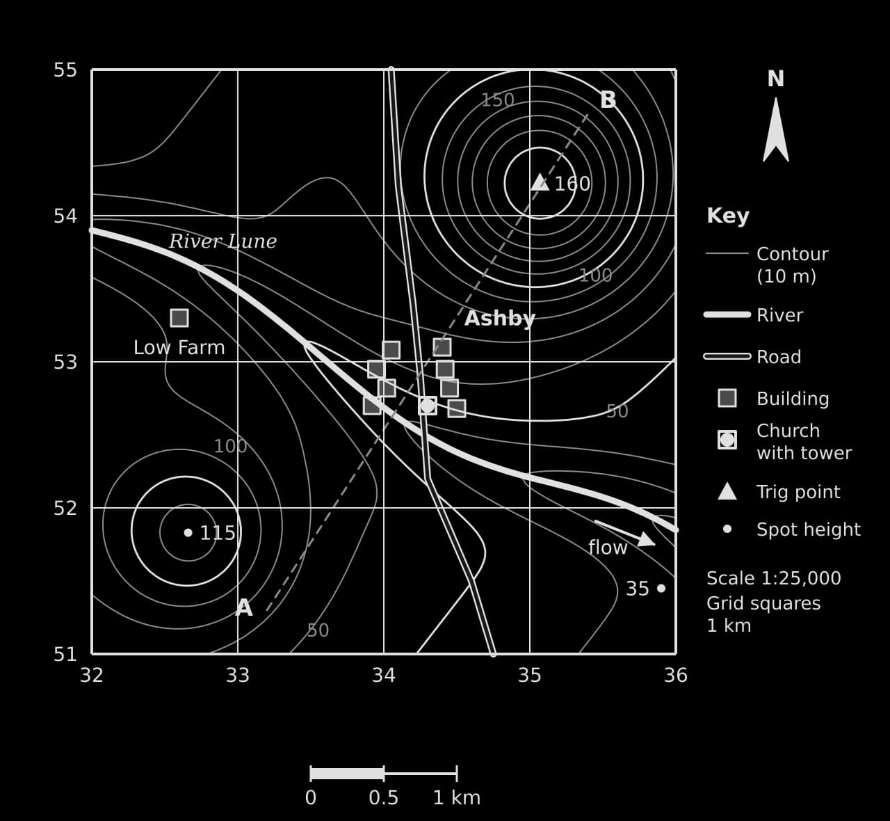
Hypothetical 1:25,000 map, eastings 32–36, northings 51–55, 10 m contours. River Lune flows east-south-east past Ashby (square 3452, church 343527) and Low Farm; trig point 160 m, spot heights 115 m and 35 m; section line A–B.Hypothetical 1:25,000 map, eastings 32–36, northings 51–55, 10 m contours. River Lune flows east-south-east past Ashby (square 3452, church 343527) and Low Farm; trig point 160 m, spot heights 115 m and 35 m; section line A–B.
A hypothetical 1:25,000 extract. The church in Ashby sits three-tenths of the way across square 3452 and seven-tenths of the way up it, so its six-figure reference is 343527. The River Lune flows east-south-east between two hills.

The map extract shows the standard features of a topographic map: a 1 km grid with eastings 32–36 and northings 51–55, contour lines at a 10 m interval, spot heights and a trig point, a river, a road, buildings and a key. The village of Ashby lies in grid square 3452, because the south-west corner of the square containing most of its buildings is where easting 34 meets northing 52.

Tip

"Along the corridor and up the stairs": read the easting along the bottom of the map first, then the northing up the side. The same rule works for every grid, from Ordnance Survey maps to the grid printed on an exam resource booklet.

Worked example

Using the map extract of Ashby: (a) State the four-figure grid reference of Low Farm. (b) State the six-figure grid reference of the trig point. (c) Identify the direction of the trig point from the church. (d) Estimate the straight-line distance from the church to the trig point.

Show the solution

(a) Low Farm lies in the square whose south-west corner is easting 32, northing 53: 3253.

(b) The trig point is on easting 35 (zero tenths east of it, so the third figure is 0) and about two-tenths of the way from northing 54 to northing 55: 350542.

(c) From the church (343527) the trig point is about 0.8 km further east and 1.5 km further north, so it lies to the north-north-east (a bearing of about 027°).

(d) Measured on the map, the distance is about 6.8 cm; at 1:25,000 that is 6.8 × 0.25 = 1.7 km. (By Pythagoras on the grid: √(0.77² + 1.52²) = 1.70 km.)

Common mistake

Giving the northing before the easting, or reading the grid line at the top or right of a square instead of the south-west corner. A four-figure reference for the square to the north-east of the lines 34 and 52 is 3452, not 3553 or 5234.

Height, relief and gradient

Relief (the shape and height of the land) is shown by contour lines, which join points of equal height above sea level, and by spot heights, which give the exact height of a single point. The contour interval is the vertical distance between adjacent contours, usually 5 m or 10 m on 1:25,000 and 1:50,000 maps; every fifth contour (an index contour) is drawn thicker and labelled.

Definition

Contour line: a line on a map joining points of equal height above sea level; the vertical distance between adjacent contours is the contour interval.

Contour pattern

What it shows

On the Ashby extract

Contours close together

Steep slope

The southern flank of the hill in squares 3553 and 3554

Contours far apart

Gentle slope or flat land

The valley floor beside the river in square 3352

Closed rings of rising value

A hill or summit

The hill topped by the trig point (160 m) and the hill with spot height 115 m

V-shapes pointing upstream (to higher ground)

A river valley

The 50 m and 60 m contours where they cross the River Lune

V-shapes or U-shapes pointing downhill

A spur (a ridge of higher land between valleys)

Not shown

Evenly spaced contours

A uniform slope

The north-west of the map in square 3254

Gradient is the steepness of a slope: the vertical rise divided by the horizontal distance, both in the same units. It can be written as a ratio ("1 in 20"), a percentage or an angle.

Gradient=vertical intervalhorizontal distanceGradient=horizontal distancevertical interval​

Worked example

On the Ashby extract, the trig point is at 160 m (350542) and the spot height in the south-east is at 35 m (359514). The straight-line distance between them is 2.89 km. Determine the average gradient between them as a ratio and as a percentage.

Show the solution

Step 1: vertical interval. 160 m − 35 m = 125 m.

Step 2: horizontal distance in the same unit. 2.89 km = 2,890 m.

Step 3: gradient. 125 ÷ 2,890 = 0.043. As a ratio, 2,890 ÷ 125 = 23.1, so about 1 in 23; as a percentage, 0.043 × 100 = 4.3% (an angle of about 2.5°).

This is an average: the slope is much steeper near the summit, where the contours are closest together, and gentler near the river.

Drawing a cross-section

A cross-section (cross-profile) is a side view of the land surface along a straight line between two points. It turns the contour pattern into a shape that can be described and compared, and it is the standard way to show a valley, a coastal slope or the position of settlements on relief.

  1. Lay the straight edge of a strip of paper along the line between the two points (A and B) and mark both ends.

  2. Mark on the strip every place where a contour crosses the edge, and write its height beside the mark. Mark rivers, roads and settlements too.

  3. Draw a horizontal axis the same length as the strip (the map’s scale) and a vertical axis for height, with a scale chosen so that the section is readable.

  4. Place the strip along the horizontal axis and plot each height above its mark. Join the points with a smooth curve, not straight lines; rivers sit at the lowest points and hilltops are rounded above the highest contour.

  5. Label A and B, the features crossed, both axes with units, and state the vertical exaggeration.

The vertical scale is almost always larger than the horizontal one; otherwise most landscapes would look flat. The vertical exaggeration is the vertical scale divided by the horizontal scale. If 1 cm represents 25,000 cm (250 m) horizontally and 20 m vertically, the vertical exaggeration is 250 ÷ 20 = 12.5.

Definition

Vertical exaggeration: the number of times the vertical scale of a cross-section is larger than its horizontal scale.

Worked example

Construct a cross-section along the line A (332513) to B (354547) on the Ashby extract, and describe the relief it shows.

Show the solution

Step 1: the line A–B measures 16.2 cm on the map, which at 1:25,000 is 4.05 km. Mark the contours it crosses: it starts at about 72 m, falls through the 70, 60 and 50 m contours to the river at about 41 m, then climbs through every contour from 50 m to 150 m and passes almost over the 160 m summit before falling to about 117 m at B.

Step 2: draw the axes (distance 0–4.05 km, height 0–180 m) and plot the heights.

Cross-section from A (72 m) to B (117 m), 4.05 km long: gentle fall to the River Lune valley floor at about 41 m 1.6 km from A, then a steep rise to a summit of about 160 m at 3.5 km and a fall to B.Cross-section from A (72 m) to B (117 m), 4.05 km long: gentle fall to the River Lune valley floor at about 41 m 1.6 km from A, then a steep rise to a summit of about 160 m at 3.5 km and a fall to B.
The section shows an asymmetrical valley: a fall of about 30 m over 1.6 km from A to the river, then a rise of about 120 m in under 2 km to the hill summit. Vertical exaggeration about × 13.

Step 3: describe. From A the land falls gently, about 30 m in 1.6 km, to the River Lune at about 41 m. East of the river the slope is much steeper: the land rises about 120 m in 1.9 km to a rounded summit at about 160 m, 3.5 km from A, then falls to 117 m at B. The valley is therefore asymmetrical, with its steeper side to the north-east.

Common mistake

Joining the points of a cross-section with straight lines, drawing the river on a slope instead of at the lowest point, or leaving out the vertical scale. A section without labelled axes and features cannot show what it is meant to show.

Thematic maps

Thematic maps show the distribution of one variable. Each type suits a particular kind of data, and choosing the wrong one gives a misleading picture. The key question is whether the data are absolute values (a number of people, visitors or migrants), relative values (a density, a rate, a percentage), or a quantity that varies continuously over space (temperature, rainfall, height).

Map type

Best for

Example

Main limitation

Choropleth

Relative values for areas (densities, rates, percentages)

Population density by district; GNI per capita by country

Implies a uniform value across each area and a sudden change at its boundary

Isoline

Quantities that vary continuously over space

Temperature, rainfall, pressure, height (contours)

Values between data points are estimated (interpolated)

Proportional symbols

Absolute values at points or for areas

City populations; tourist arrivals

Large symbols overlap; areas are hard to judge by eye

Dot map

The location of individual features or counts

Shops, wells, cases of a disease

Dots merge in dense areas; one dot may stand for many features

Flow-line

Movements between places

Migration, trade, commuting, traffic

Routes are simplified; many flows clutter the map

Choropleth maps

A choropleth map shades each area (a country, region or district) according to the class its value falls into, in graded tones of one colour from light (low) to dark (high). It shows relative data well: population per km², the percentage of people over 65, or GDP per capita. It should not be used for absolute numbers, because a large area will look important simply because it is large.
Definition

Choropleth map: a map that shades areas in graded tones of one colour according to classes of a relative value, such as a density, rate or percentage.

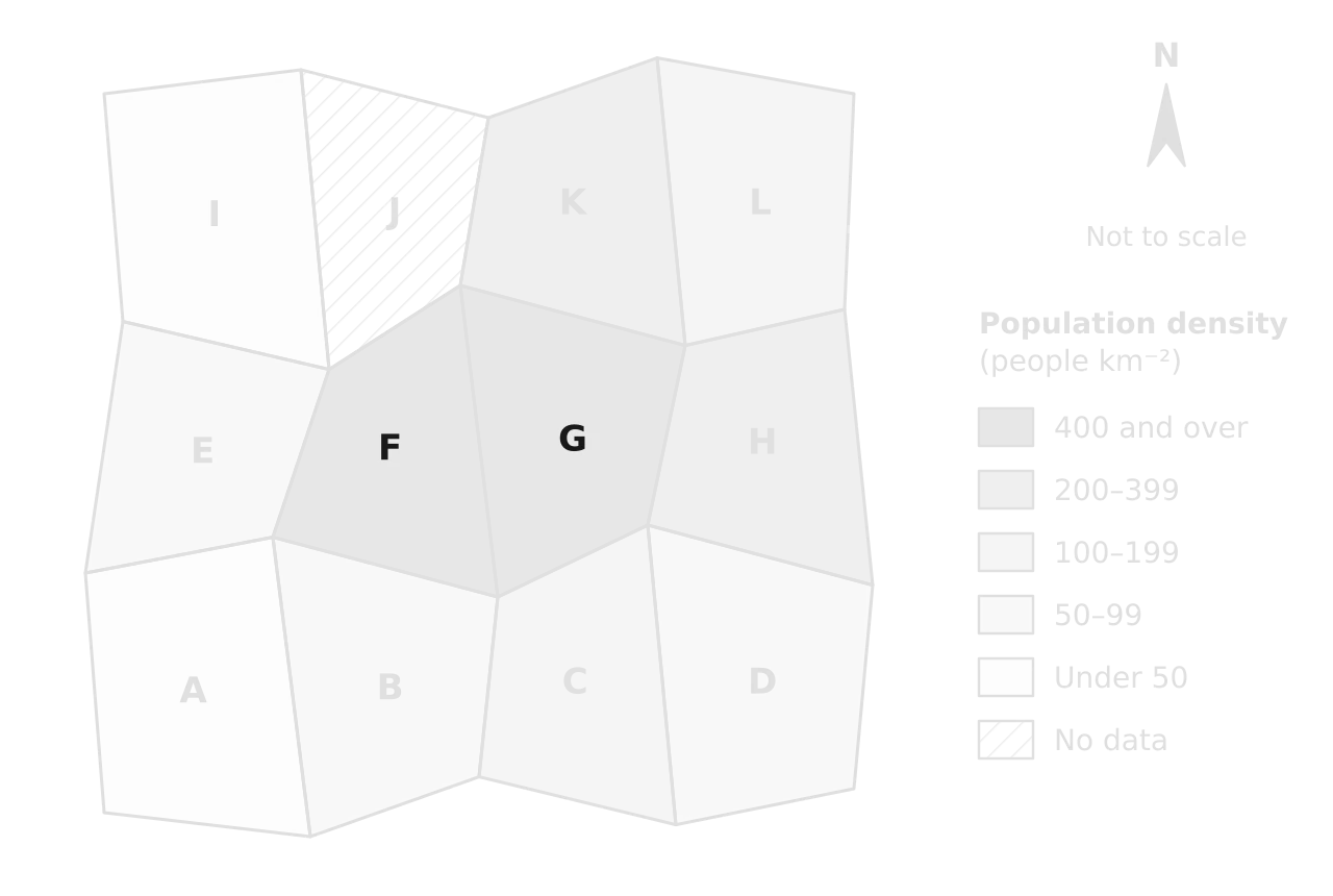
Choropleth of 12 hypothetical districts A–L shaded in five classes of population density from under 50 to 400 and over people per km², with district J hatched as no data. Densities are highest in central districts F and G.Choropleth of 12 hypothetical districts A–L shaded in five classes of population density from under 50 to 400 and over people per km², with district J hatched as no data. Densities are highest in central districts F and G.
Population density is highest in the central districts F and G and falls towards the edges of the region. G (1,260 people km⁻²) and F (410) share one class, so the map hides a threefold difference between them.

To construct a choropleth map, decide on four to six classes that cover the data without gaps or overlaps (under 50, 50–99, 100–199 and so on), give each a tone that becomes darker as values rise, shade each area, and add a key with the class intervals and a "No data" class where values are missing. Class boundaries can be equal steps, steps that double, or natural breaks in the data; changing them can make the same data look quite different, which is why the key matters.

Worked example

District F of the region has a population of 1,230,000 and an area of 3,000 km². (a) Determine its population density and identify its class on the choropleth map. (b) Describe the distribution of population density shown on the map.

Show the solution

(a) Population density = population ÷ area = 1,230,000 ÷ 3,000 km² = 410 people per km², which falls in the darkest class, "400 and over".

(b) The highest densities (400 and over people per km²) are in the two central districts, F and G, and moderately high densities (200–399) in the districts east and north-east of them (H and K). Densities fall towards the edges: the south-western district A and the north-western district I have under 50 people per km². The pattern is broadly a central core with lower densities around it, and there is no data for district J.

Common mistake

Shading absolute numbers on a choropleth map, or using several unrelated colours for the classes. A choropleth map shows rates or densities in tones of one colour, darker for higher values; absolute numbers belong on a proportional symbol map.

Isoline maps

An isoline map joins places of equal value of a quantity that changes gradually over space. Contours are isolines of height; isotherms join equal temperatures, isohyets equal rainfall and isobars equal pressure. Isolines are drawn by interpolation: estimating values between measured points and threading a line through where the chosen value would fall. They never cross, and close spacing shows a steep gradient in the variable.
Definition

Isoline map: a map with lines joining places of equal value of a continuously varying quantity, such as temperature (isotherms), rainfall (isohyets) or pressure (isobars).

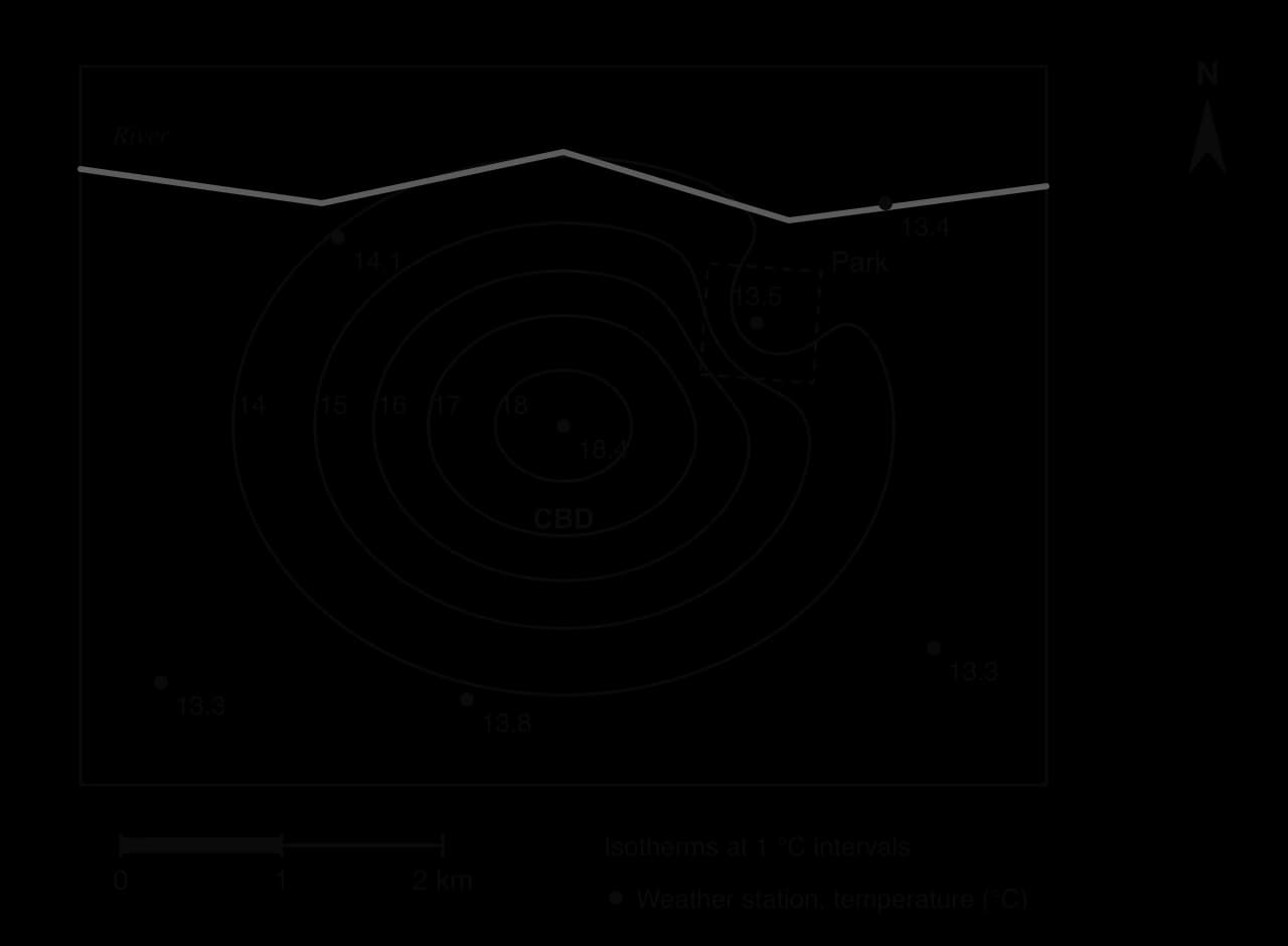
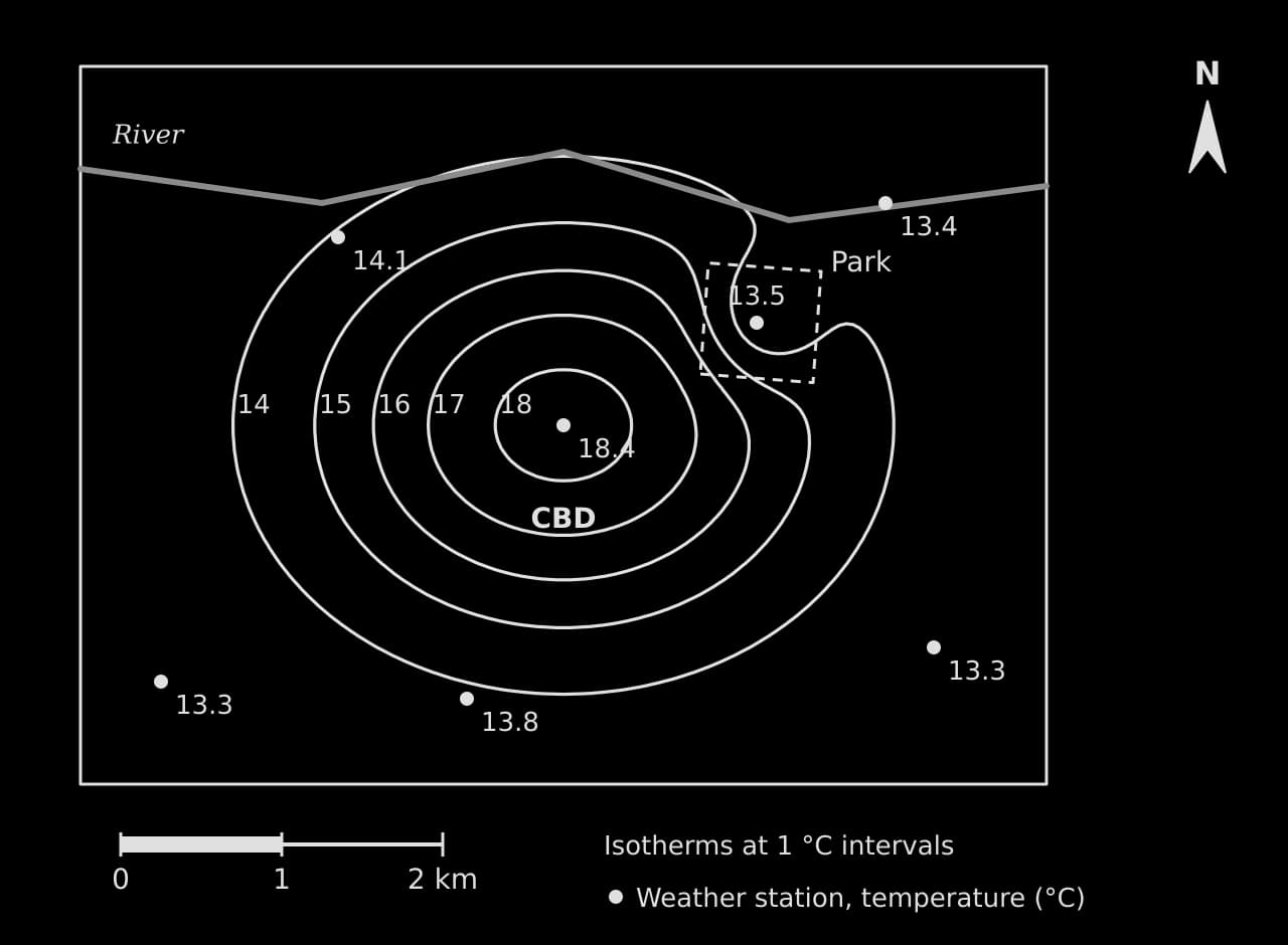
Isoline map of a hypothetical city at night: closed isotherms from 14 to 18 °C around the CBD (18.4 °C), bending inward around a cooler park (13.5 °C); rural stations 13.3–13.8 °C; river to the north; scale bar 2 km.Isoline map of a hypothetical city at night: closed isotherms from 14 to 18 °C around the CBD (18.4 °C), bending inward around a cooler park (13.5 °C); rural stations 13.3–13.8 °C; river to the north; scale bar 2 km.
The closed isotherms show an urban heat island: night-time air is 18.4 °C at the CBD station and 13.3–13.8 °C at the rural stations. The isotherms bend inward around the park, where vegetation keeps the air cooler.

The isoline map shows an urban heat island, a common fieldwork and exam topic: temperatures rise towards the central business district and fall towards the rural edge, and the intensity of the heat island is the difference between the two, here 18.4 − 13.3 = 5.1 °C. A place halfway between the 16 °C and 17 °C isotherms is estimated at 16.5 °C.

Proportional symbol maps

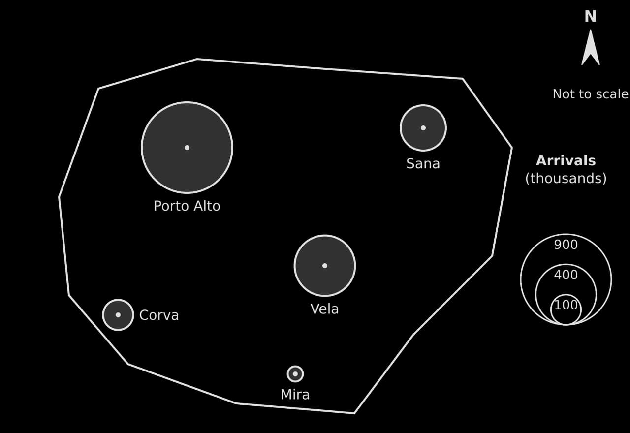
A proportional symbol map places a symbol, usually a circle, at each location and draws it with its area proportional to the value there. Because the area of a circle is πr², the radius must be proportional to the square root of the value: a town with four times the visitors of another has a circle twice as wide, not four times as wide.
r=kvr=kv​
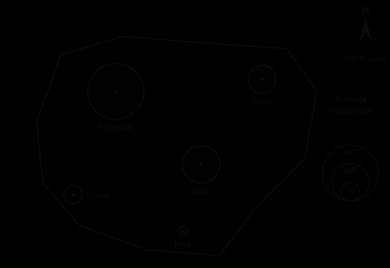
Proportional circles on a hypothetical island: tourist arrivals Porto Alto 900, Vela 400, Sana 225, Corva 100 and Mira 25 thousand; circle areas proportional to arrivals; nested key circles for 900, 400 and 100 thousand.Proportional circles on a hypothetical island: tourist arrivals Porto Alto 900, Vela 400, Sana 225, Corva 100 and Mira 25 thousand; circle areas proportional to arrivals; nested key circles for 900, 400 and 100 thousand.
Porto Alto has 900,000 arrivals, nine times as many as Corva (100,000), so its circle has three times the radius. The nested key lets the reader estimate values by comparing sizes.

Worked example

On a proportional circle map, 100,000 tourist arrivals are drawn as a circle of radius 5 mm. Determine the radius for towns with 900,000, 400,000 and 25,000 arrivals.

Show the solution

Step 1: find k. r = k√v. With v in thousands, 5 mm = k × √100 = 10k, so k = 0.5 mm.

Step 2: apply it. 900 thousand: 0.5 × √900 = 0.5 × 30 = 15 mm. 400 thousand: 0.5 × 20 = 10 mm. 25 thousand: 0.5 × 5 = 2.5 mm.

Step 3: check. 900,000 is nine times 100,000 and its radius is three times larger, so the area is nine times larger, as it should be.

Dot maps

A dot map shows a distribution by placing a dot for each feature (a shop, a well, a case of a disease) or for a fixed number of them (one dot for 1,000 people). It shows clustering and spacing directly, which makes it the starting point for the nearest neighbour index, a measure of whether the pattern is clustered, random or regular.

To construct a dot map, choose what one dot represents, place each dot where the features occur rather than in the middle of an area, and state the dot value in the key. Its main weakness is that dots merge where they are dense, so the value per dot must be chosen with the densest area in mind.

Flow-line maps

A flow-line map shows movement between places, such as migration, trade, commuting or traffic. The direction of each arrow shows the route, and its width is proportional to the volume of the flow, read against a key of reference widths. Flow lines can follow real routes or be drawn as straight lines from origin to destination. To construct one, choose a width scale (for example 3 mm for every 1,000 migrants), draw each arrow from origin to destination at its width, and show two or three reference widths in the key.
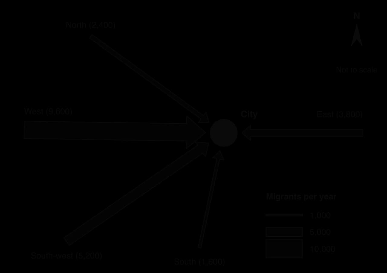
Flow-line map of migrants into a hypothetical city: arrows from West 9,600, South-west 5,200, East 3,800, North 2,400 and South 1,600 per year, each arrow's width proportional to the number; key shows widths for 1,000, 5,000 and 10,000.Flow-line map of migrants into a hypothetical city: arrows from West 9,600, South-west 5,200, East 3,800, North 2,400 and South 1,600 per year, each arrow's width proportional to the number; key shows widths for 1,000, 5,000 and 10,000.
The widest flow, from the West (9,600 migrants), carries over 40% of the 22,600 arrivals; the North and South send fewest. The key’s reference widths allow each flow to be estimated.

Worked example

Using the flow-line map, (a) state the region that sends the most migrants to the city, and (b) determine its share of all arrivals.

Show the solution

(a) The West (9,600 migrants per year).

(b) Total arrivals = 9,600 + 5,200 + 3,800 + 2,400 + 1,600 = 22,600. Share = 9,600 ÷ 22,600 × 100 = 42.5%.

Topological maps, mental maps and sketch maps

A topological map keeps only the connections between places and their order, not true distances or shapes; the London Underground map is the classic example, and network diagrams of air routes or shipping lanes work in the same way. Lines are straightened, stations are spaced evenly and interchanges are emphasised, so the map is easy to follow but cannot be used to measure distance or direction.
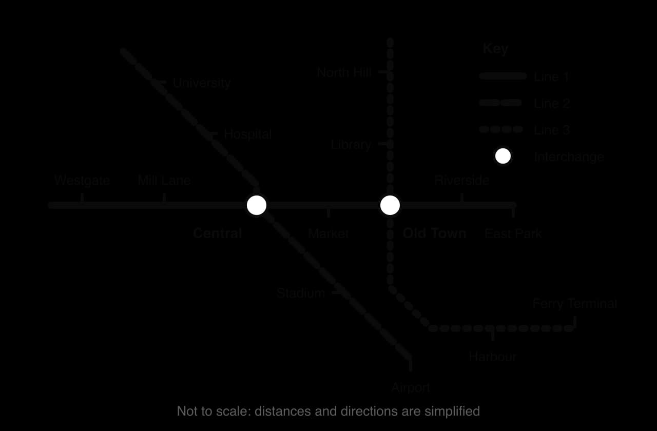
Topological map of a hypothetical metro: Line 1 west–east, Line 2 north-west to south-east, Line 3 north–south then east to Ferry Terminal; interchanges at Central and Old Town; 13 other stations; straight lines, not to scale.Topological map of a hypothetical metro: Line 1 west–east, Line 2 north-west to south-east, Line 3 north–south then east to Ferry Terminal; interchanges at Central and Old Town; 13 other stations; straight lines, not to scale.
Only the order of stations and the connections between lines are shown. Central and Old Town are the interchanges; the even spacing hides how far apart the stations really are. Hypothetical network.

To read a topological map, follow the lines and count stops or links, not kilometres: the number of connections a place has measures its accessibility within the network. A mental map is the map of an area that a person carries in their head, often drawn in fieldwork to compare how different groups perceive a city. A sketch map is a simple map drawn by the geographer to locate the features in an answer or a report.

Tip

Every sketch map, however rough, needs five things: a title, a north arrow, a scale bar or "not to scale", a key for any symbols, and labels for the places named in the text.

Every map is a selection. The person who makes it decides what to show, which classes to use, which projection to draw it on and what to leave out, so the same data can be made to look alarming or reassuring. A geographer reading a map asks who made it, for what purpose and what it omits, in the same way as when reading a text.

Graphs and diagrams

A graph is the right choice when it makes a pattern easier to see than a table of the same numbers. The type depends on the data: time series suit line graphs, categories suit bar graphs, parts of a whole suit compound bars or pie charts, and a relationship between two variables suits a scatter graph. Several geographical graphs (triangular graphs, rose diagrams, Lorenz curves, population pyramids) exist for one particular kind of data.

Data

Graph

Construction rules

Main limitation

Change over time (continuous)

Line graph

Time on the x-axis at even intervals; points joined; several lines told apart by style and a key

Joining points implies steady change between readings; a stretched y-axis exaggerates trends

Values for separate categories

Bar graph

Bars of equal width with gaps; ordered by size or category; axis from zero

Compares one variable at a time unless bars are grouped

Parts of a total for several places or years

Compound bar graph

Components in the same order in every bar; key; often as percentages of 100

Only the bottom component starts from a common baseline, so the others are hard to compare

Parts of one total

Pie chart

Each sector = share × 360°; at most six or seven sectors; largest first

Small differences between sectors are hard to judge; poor for change over time

Two variables measured at the same sites

Scatter graph

Independent variable on the x-axis; best-fit line only if a trend exists

Shows a relationship, not its cause

Three percentages adding to 100%

Triangular graph

Read each axis along its gridlines

Only for three components; easy to misread without practice

Data spanning several orders of magnitude

Logarithmic graph

Log axis labelled with powers of ten; caption says so

Easily read as linear; cannot show zero or negative values

Frequency by direction

Rose diagram

North at the top; petal length proportional to frequency; scale rings

Directions grouped into 8 or 16 classes; hides change through the year

Scores between two opposites

Bipolar graph

Criteria listed; scale from negative to positive with zero marked

Scores are subjective judgments

Age and sex structure

Population pyramid

Males left, females right; five-year cohorts; % or absolute numbers

A snapshot of one year; percentages hide the total population

Income or resource distribution

Lorenz curve

Cumulative percentages on both axes; line of perfect equality

Shows how evenly income is shared, not how high it is

Line, bar and compound bar graphs

Line graphs show continuous change, such as population over time or discharge over a storm. Bar graphs compare separate categories, such as rainfall by month or visitors by country of origin. Both need a title, labelled axes with units, a scale that starts at zero on bar graphs, and a key when there is more than one series.

A climate graph combines the two on one set of axes: monthly rainfall as bars against the left-hand axis and mean monthly temperature as a line against the right-hand axis. Rainfall is drawn as bars because each month’s total is a separate quantity; temperature is a line because it changes continuously through the year.
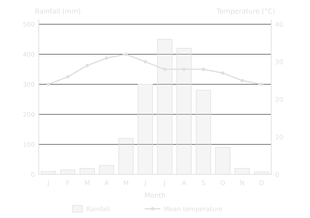
Climate graph of a hypothetical monsoon city: rainfall bars from 8 mm in December to 450 mm in July, very wet June–September; temperature line from 24 °C in January to a peak of 32 °C in May, falling to 28 °C in the rainy months.Climate graph of a hypothetical monsoon city: rainfall bars from 8 mm in December to 450 mm in July, very wet June–September; temperature line from 24 °C in January to a peak of 32 °C in May, falling to 28 °C in the rainy months.
Almost all the rain falls from June to September, with a peak of 450 mm in July, while temperature peaks at 32 °C in May, just before the rains, and falls slightly under the cloud of the wet season. Hypothetical data.

Worked example

Using the climate graph, (a) identify the wettest month, (b) determine the total annual rainfall and the annual temperature range, and (c) determine the percentage of the year’s rain that falls from June to September.

Show the solution

(a) July, with 450 mm.

(b) Total rainfall = 10 + 15 + 20 + 30 + 120 + 300 + 450 + 420 + 280 + 90 + 20 + 8 = 1,763 mm. Temperature range = maximum − minimum = 32 °C − 24 °C = 8 °C.

(c) June to September = 300 + 450 + 420 + 280 = 1,450 mm; 1,450 ÷ 1,763 × 100 = 82% of the annual total. Read from a printed graph, the values are estimates, so answers within a few millimetres of each bar are accepted.

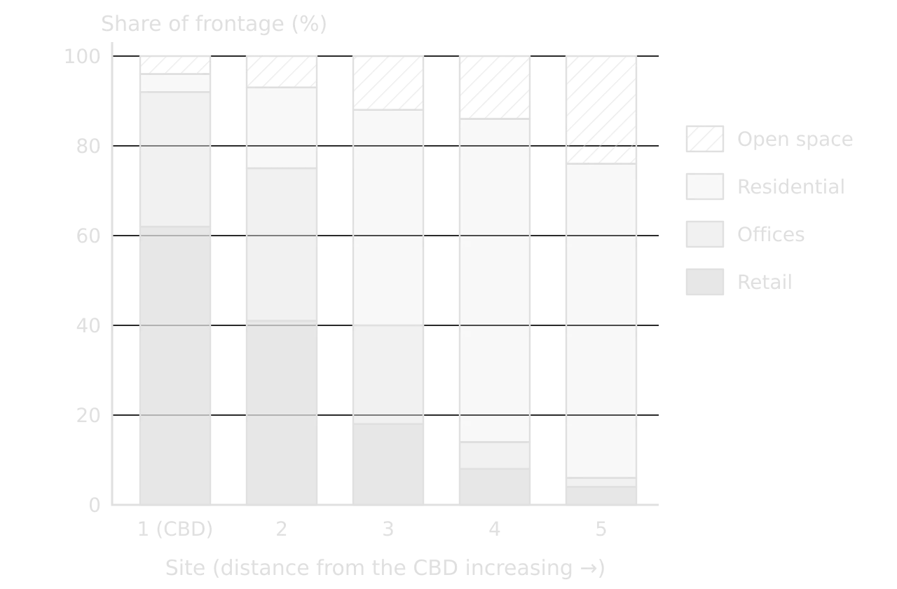
A compound bar graph divides each bar into the components of a total, so it shows both the total and its make-up. Drawn as percentages, every bar reaches 100% and only the shares change. It is widely used in fieldwork for land use, the types of shops in a street, or the modes of transport people use.
Definition

Compound bar graph: a bar graph in which each bar is divided into the components of a total, shown either as values or as percentages of 100.

Compound bar graph of land use at five sites from the CBD outwards: retail falls from 62% to 4%, offices from 30% to 2%, residential rises from 4% to 70%, open space from 4% to 24% (hypothetical).Compound bar graph of land use at five sites from the CBD outwards: retail falls from 62% to 4%, offices from 30% to 2%, residential rises from 4% to 70%, open space from 4% to 24% (hypothetical).
Retail and offices dominate the frontage at the CBD (92% together) and almost disappear by site 5 (6%), while residential land rises from 4% to 70% and open space from 4% to 24% (hypothetical survey).

The compound bar graph summarises a land-use transect from the city centre. Its pattern matches the idea of a central commercial core surrounded by residential zones: the share of commercial land falls steadily with distance, and residential land takes over between sites 2 and 3. A pie chart for each site would show the same data but make the change between sites much harder to compare.

Pie charts

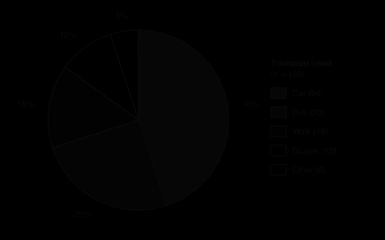
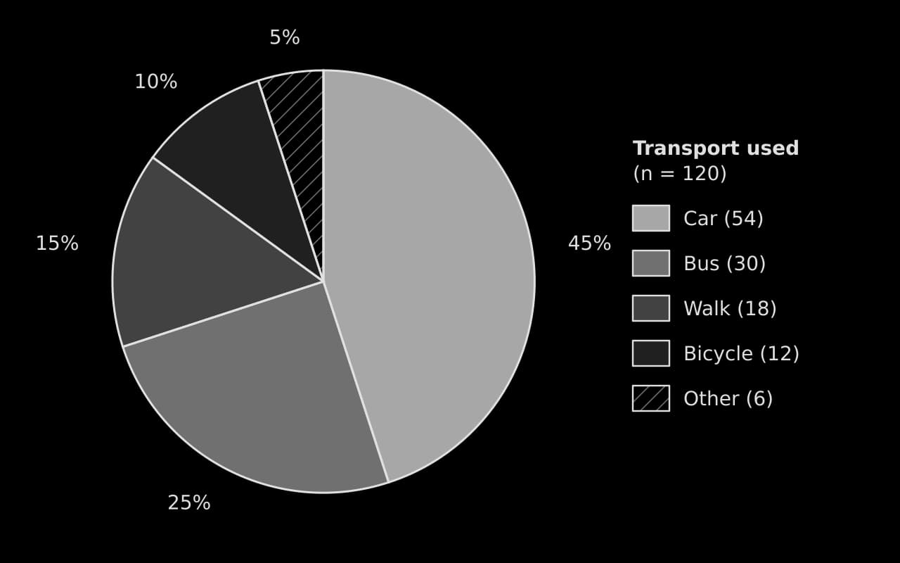
A pie chart shows how one total is divided between categories, each drawn as a sector whose angle is proportional to its share. It suits a single place or year with a few categories, such as the transport used by shoppers or the land use of one survey area. Sectors are drawn clockwise from the top, largest first, with "other" last, and labelled with percentages.
Worked example

In a questionnaire, 120 shoppers said how they travelled to a town centre: car 54, bus 30, walking 18, bicycle 12 and other 6 (hypothetical data). Determine the angle of each sector for a pie chart.

Show the solution

Step 1: degrees per person. 360° ÷ 120 = 3° per respondent.

Step 2: angles. Car 54 × 3 = 162°; bus 30 × 3 = 90°; walking 18 × 3 = 54°; bicycle 12 × 3 = 36°; other 6 × 3 = 18°. Check: 162 + 90 + 54 + 36 + 18 = 360°.

Step 3: percentages for the labels. Car 54 ÷ 120 × 100 = 45%; bus 25%; walking 15%; bicycle 10%; other 5%.

Pie chart of how 120 shoppers travelled to a town centre (hypothetical): car 54 (45%), bus 30 (25%), walk 18 (15%), bicycle 12 (10%), other 6 (5%), sectors drawn clockwise from the top, largest first.Pie chart of how 120 shoppers travelled to a town centre (hypothetical): car 54 (45%), bus 30 (25%), walk 18 (15%), bicycle 12 (10%), other 6 (5%), sectors drawn clockwise from the top, largest first.
Cars bring 45% of shoppers and buses 25%, so motor vehicles account for 70% of trips; walking and cycling together make up a quarter. Hypothetical questionnaire of 120 shoppers.

Scatter graphs

A scatter graph plots two variables measured at the same places, such as distance downstream and channel width, or GNI per capita and life expectancy. The independent variable, the one thought to cause the change, goes on the x-axis. If the points form a band, a best-fit line can be drawn by eye through the middle of them, with about as many points above as below; it does not have to pass through the origin or through any point.
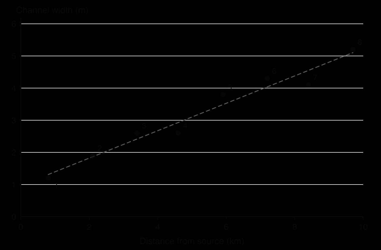
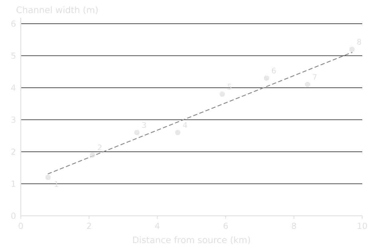
Scatter graph of channel width (m) against distance from source (km) for eight sites: width rises from 1.2 m at 0.8 km to 5.2 m at 9.7 km, close to a dashed best-fit line; sites 3 and 4 both 2.6 m.Scatter graph of channel width (m) against distance from source (km) for eight sites: width rises from 1.2 m at 0.8 km to 5.2 m at 9.7 km, close to a dashed best-fit line; sites 3 and 4 both 2.6 m.
Distance downstream is the independent variable, so it goes on the x-axis. The points lie close to a best-fit line, a strong positive correlation; sites 4 and 7 sit slightly below it. Hypothetical river data.

The pattern describes the correlation: positive if both variables rise together, negative if one falls as the other rises, and none if there is no trend. A tight band is a strong correlation, a loose cloud a weak one. Points far from the line are anomalies and need explaining. Spearman’s rank correlation coefficient measures the strength of the relationship and tests whether it could have arisen by chance.

Common mistake

Treating a correlation as proof of cause. Two variables can rise together because both depend on a third (ice cream sales and drowning both rise in hot weather). A scatter graph can show only that a relationship exists; geographical theory is needed to explain it.

Triangular graphs

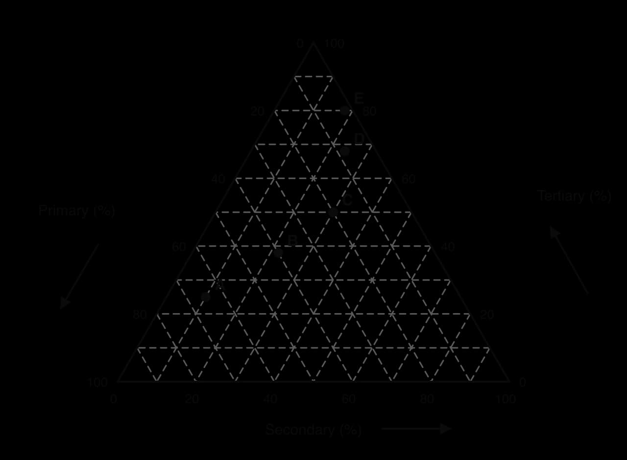
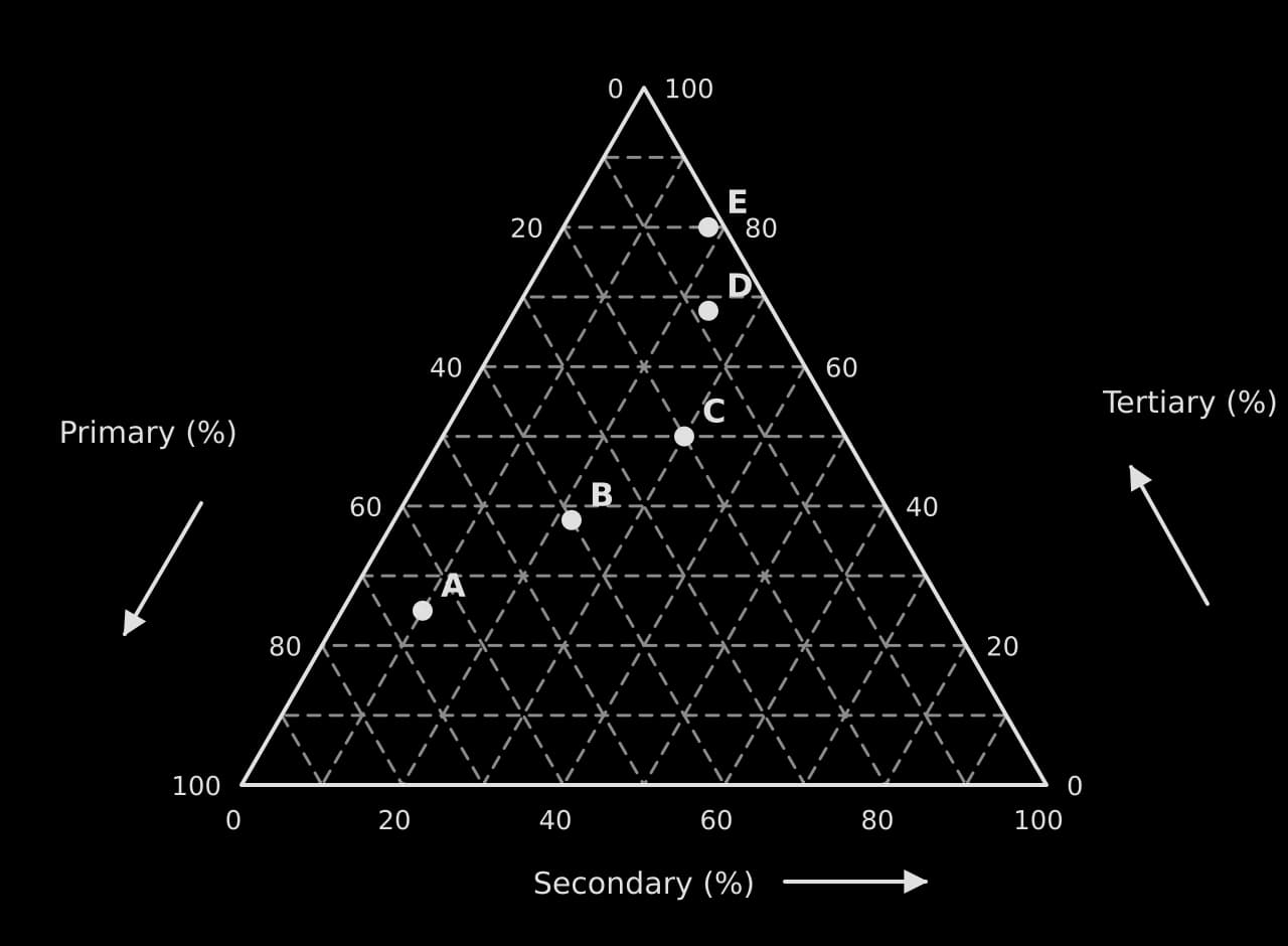
A triangular graph plots data made of three percentages that add up to 100%, such as employment in the primary sector, secondary sector and tertiary sector, or the sand, silt and clay in a soil. Each side of the triangle is a 0–100% axis for one component, and each point represents one place.
Definition

Triangular graph: a graph shaped as an equilateral triangle that plots data made of three percentage components adding to 100%.

Triangular graph of primary, secondary and tertiary employment (%) with 10% gridlines; countries A (65, 10, 25), B (40, 22, 38), C (20, 30, 50), D (8, 24, 68) and E (2, 18, 80) plotted; arrows show the reading direction on each axis.Triangular graph of primary, secondary and tertiary employment (%) with 10% gridlines; countries A (65, 10, 25), B (40, 22, 38), C (20, 30, 50), D (8, 24, 68) and E (2, 18, 80) plotted; arrows show the reading direction on each axis.
The five countries form a line from A (65% of workers in the primary sector) to E (80% in the tertiary sector). This shift in employment structure is what the Clark–Fisher model describes as countries develop.

Reading a triangular graph is easiest one axis at a time. For each component, find the gridlines that run parallel to the side opposite that component’s 100% corner, follow the line through the point to the axis, and read the value in the direction of the arrow. The three readings must add up to 100%, which is a quick check that each has been read correctly.

Worked example

Using the triangular graph, (a) state the percentage of workers in each sector in country C, and (b) describe the change in employment structure from country A to country E.

Show the solution

(a) Country C: primary 20%, secondary 30%, tertiary 50% (check: 20 + 30 + 50 = 100).

(b) From A to E, the share of primary employment falls from 65% to 2%, and the share of tertiary employment rises from 25% to 80%. Secondary employment first rises, from 10% in A to a peak of 30% in C, and then falls to 18% in E. The points form a curved line from the primary corner towards the tertiary corner.

A full-mark description gives the direction of change, figures for the start and end, and the exception (here the rise and fall of secondary employment).

Logarithmic graphs

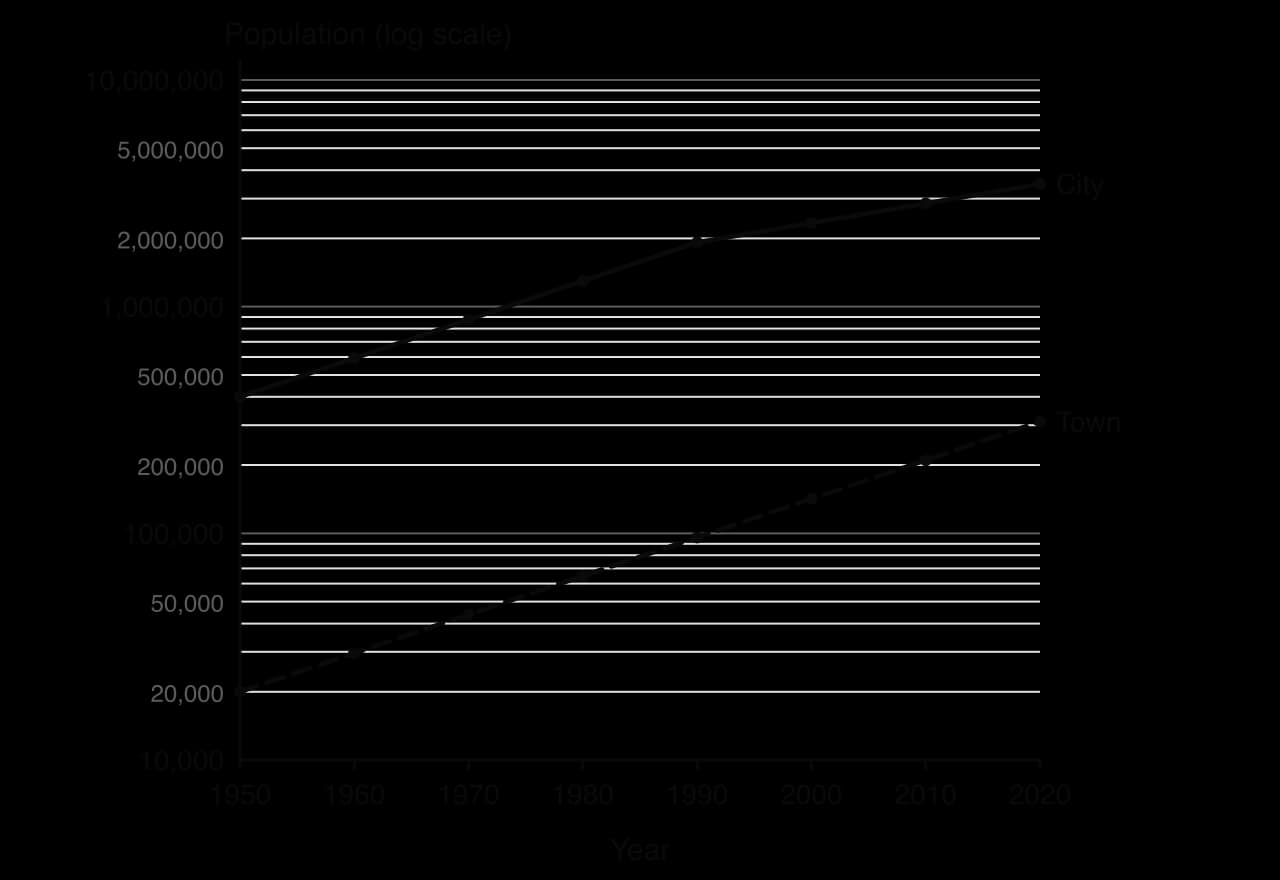
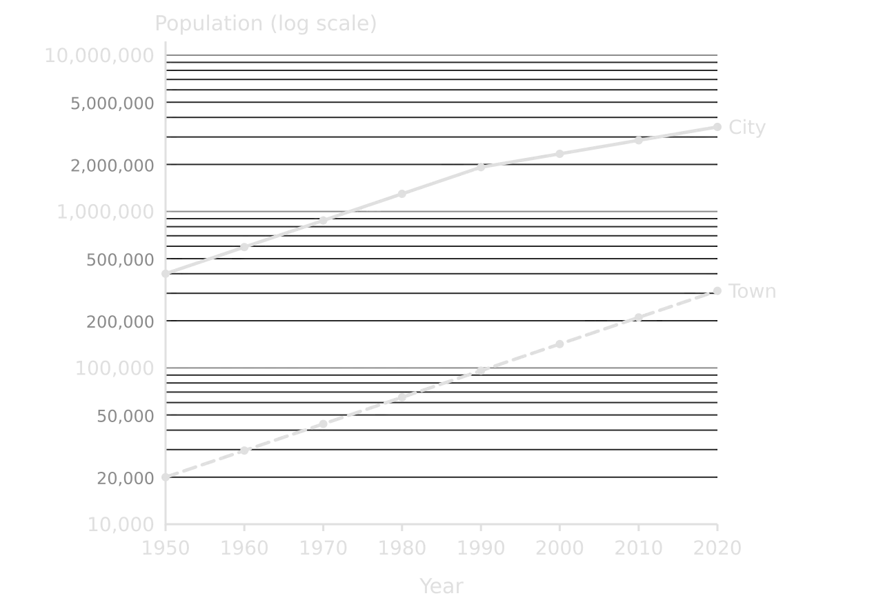
A logarithmic scale has equal distances for each tenfold increase (10, 100, 1,000, 10,000), so data with a very wide range fit on one graph: villages and megacities, or the GNI per capita of the poorest and richest countries. Between the main gridlines, the minor lines for 2, 3, 4 … 9 get closer together. A semi-logarithmic graph has one log axis; a log-log graph has two.
Definition

Logarithmic scale: a graph scale on which each equal distance represents a tenfold increase; a constant rate of growth plots as a straight line.

Semi-log graph 1950–2020, y axis 10,000 to 10,000,000 on a log scale. City grows from 400,000 to 1.92 million by 1990 then more slowly to 3.48 million; town grows steadily from 20,000 to 311,300 as a straight line.Semi-log graph 1950–2020, y axis 10,000 to 10,000,000 on a log scale. City grows from 400,000 to 1.92 million by 1990 then more slowly to 3.48 million; town grows steadily from 20,000 to 311,300 as a straight line.
On a logarithmic axis, a steady growth rate is a straight line. The town and the city both grew by about 4% a year until 1990, so their lines are parallel; after 1990 the city’s line flattens because its growth slowed to about 2% a year. Hypothetical data; y axis logarithmic.

The most useful property of a logarithmic graph is that the slope shows the rate of change, not the absolute change. On a normal axis, the city would appear to grow much faster than the town because it adds more people each year; on a log axis, the two lines are parallel from 1950 to 1990 because both grew at the same percentage rate.

Worked example

Using the semi-logarithmic graph, (a) estimate the population of the city in 1990, and (b) determine the percentage change in its population between 1950 and 1990 and between 1990 and 2020.

Show the solution

(a) The point for 1990 lies just below the 2,000,000 line: about 1.9 million (the data value is 1,920,000).

(b) 1950–1990: (1,920,000 − 400,000) ÷ 400,000 × 100 = +380%. 1990–2020: (3,478,000 − 1,920,000) ÷ 1,920,000 × 100 = +81%.

Reading values between the gridlines of a log scale needs care: the line halfway between 1,000,000 and 10,000,000 is about 3,160,000, not 5,500,000.

Common mistake

Reading a logarithmic axis as if it were linear, or describing a straight line on a semi-log graph as "constant growth in numbers". A straight line on a log axis means a constant rate of growth, so the numbers added each year increase.

Rose diagrams

A rose diagram shows how often something comes from or points in each compass direction. Each petal points in one direction and its length is proportional to the frequency; rings show the scale, and calm days (for wind) are written in the centre circle. Rose diagrams are used for wind direction, which controls wave approach and longshore drift, for the orientation of cirques or drumlins, and for the direction of pebbles’ long axes in a till deposit.
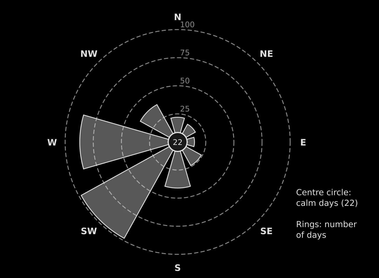
Rose diagram of wind direction in one year at a hypothetical coastal station: SW 98 days, W 87, S 41, NW 38, SE 24, N 22, NE 18, E 15; 22 calm days in the centre circle; rings at 25, 50, 75 and 100 days.Rose diagram of wind direction in one year at a hypothetical coastal station: SW 98 days, W 87, S 41, NW 38, SE 24, N 22, NE 18, E 15; 22 calm days in the centre circle; rings at 25, 50, 75 and 100 days.
The prevailing wind is from the south-west (98 days) and west (87 days): together just over half the year. Winds from the east and north-east are rare. Hypothetical data for one year.

Worked example

Using the rose diagram, (a) identify the prevailing wind direction, and (b) determine the percentage of the year with winds from the south-west or west. (c) Suggest one effect of this wind pattern on a beach facing south-west.

Show the solution

(a) South-westerly (98 days).

(b) (98 + 87) ÷ 365 × 100 = 50.7% of the year.

(c) Waves driven by the dominant south-westerly winds approach the beach most often from the south-west ✓, so if the beach is slightly oblique to them longshore drift will move sediment consistently in one direction along the coast ✓.

Bipolar graphs

A bipolar graph plots scores on a scale between two opposite descriptions, typically from −3 (poor) to +3 (good). It is the usual way to present an environmental quality survey, in which each site is scored on criteria such as litter, noise and building condition. Lines for different sites can be compared criterion by criterion, and the scores can be totalled to give each site an overall index.
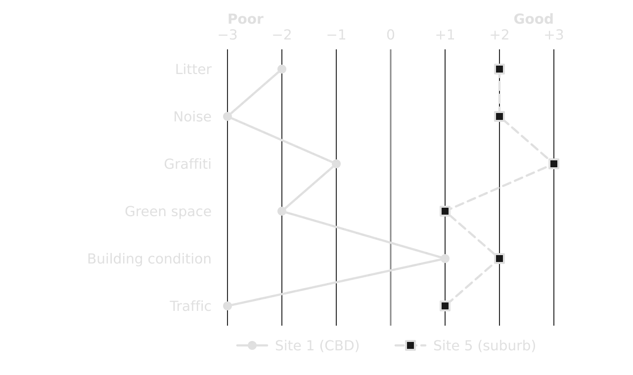
Bipolar graph of environmental quality scores from −3 (poor) to +3 (good) on six criteria. Site 1 in the CBD scores −2, −3, −1, −2, +1, −3; Site 5 in a suburb scores +2, +2, +3, +1, +2, +1 (hypothetical).Bipolar graph of environmental quality scores from −3 (poor) to +3 (good) on six criteria. Site 1 in the CBD scores −2, −3, −1, −2, +1, −3; Site 5 in a suburb scores +2, +2, +3, +1, +2, +1 (hypothetical).
The CBD site scores poorly on noise, traffic and litter but well on building condition; the suburban site scores positively on every criterion. Totals: −10 at site 1 and +11 at site 5 (hypothetical survey).

Population pyramids

A population pyramid is a pair of horizontal bar graphs, males on the left and females on the right, showing the share of the population in each five-year age group. Its shape summarises a country’s demographic history: a wide base means high fertility, a narrow base low fertility, a wide top an ageing population, and an indentation or bulge a past event such as a war, a baby boom or a wave of migration.
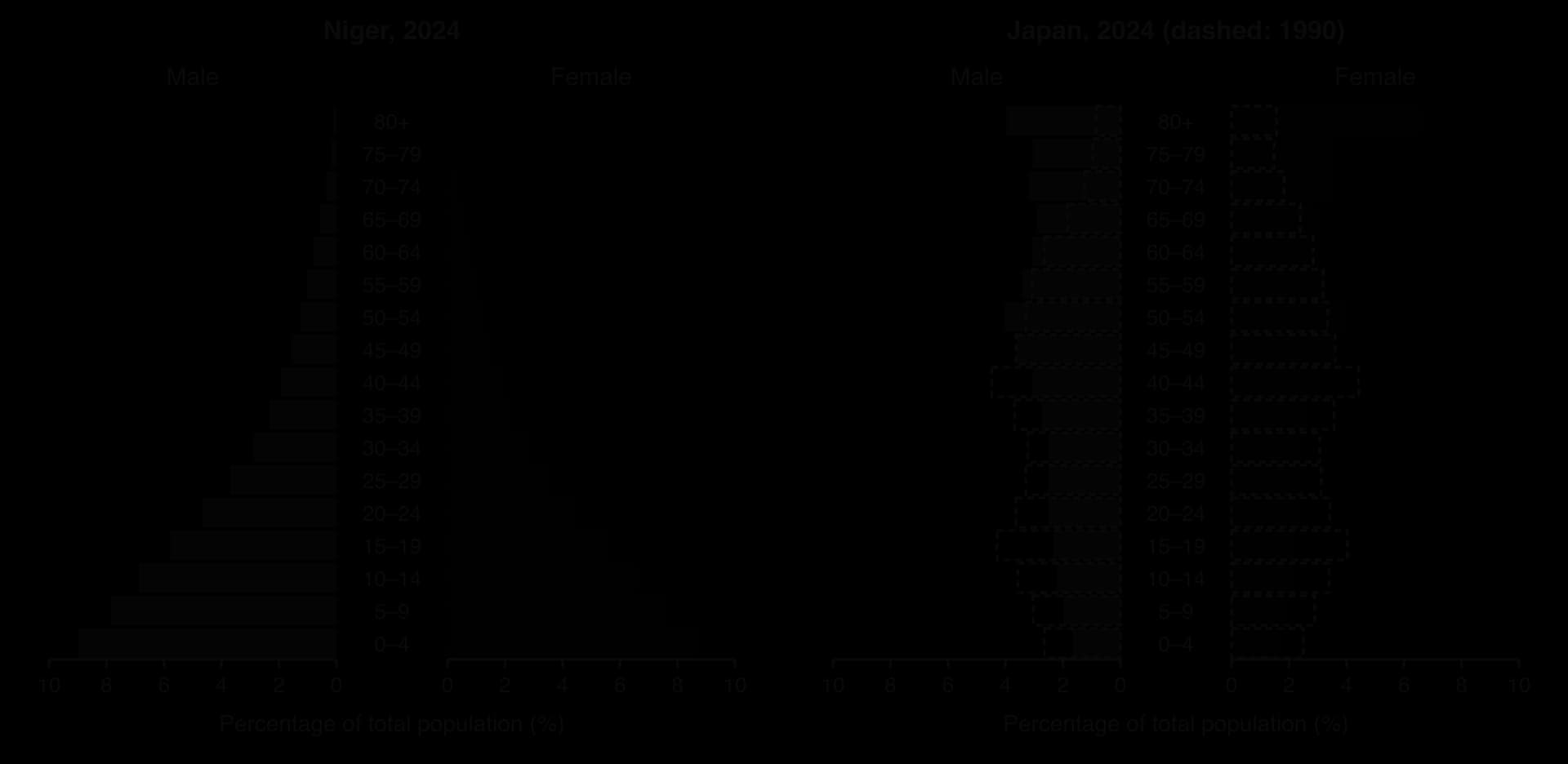
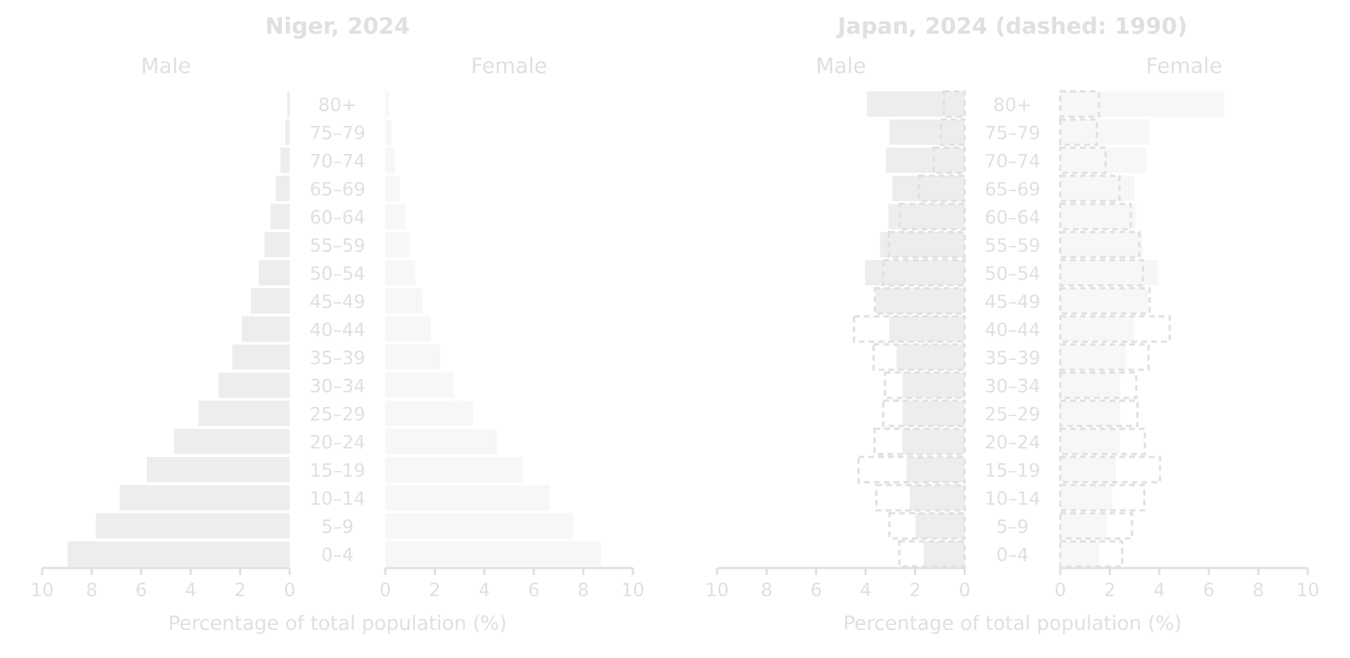
Two population pyramids on the same scale for 2024. Niger: very wide base, about 9% of the population in each sex aged 0–4, tapering sharply. Japan: narrow base under 2%, widest at 50–54, women aged 80+ 6.6%; Japan 1990 shown dashed with a wider base.Two population pyramids on the same scale for 2024. Niger: very wide base, about 9% of the population in each sex aged 0–4, tapering sharply. Japan: narrow base under 2%, widest at 50–54, women aged 80+ 6.6%; Japan 1990 shown dashed with a wider base.
Niger’s wide base shows high fertility; Japan’s narrow base and wide top show low fertility and a long life expectancy. On the same scale, the two pyramids can be compared cohort by cohort. Source: World Bank from UN WPP, 2024.

When describing a pyramid, start with the overall shape, then quantify the base and top ("about 9% of the population in each sex is aged 0–4"), then any irregularities and any difference between males and females in the oldest groups, where women usually outnumber men. A pyramid also gives the data for the dependency ratio, the number of people aged 0–14 and 65 and over for every 100 aged 15–64.

Development diamonds

A development diamond compares places on four indicators at once. Each axis runs outwards from a centre, with each indicator scaled from 0 to 100 so that outward always means "more developed" (for an indicator such as infant mortality, the scale is reversed). The larger and more regular the diamond, the higher and more balanced the level of development.
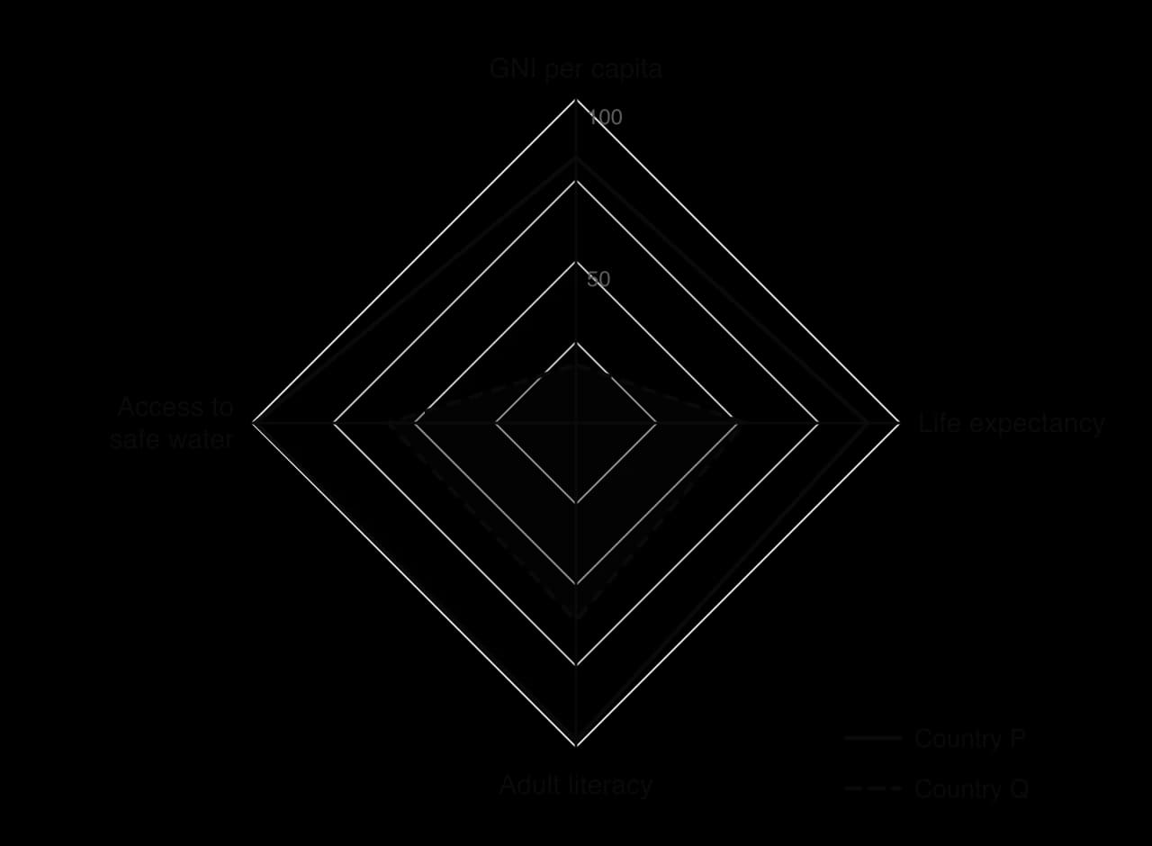
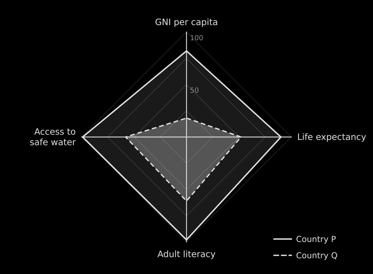
Development diamond with four axes scaled 0–100: GNI per capita, life expectancy, adult literacy and access to safe water. Country P (82, 90, 98, 99) forms a large diamond; country Q (18, 52, 61, 58) a small one, dashed.Development diamond with four axes scaled 0–100: GNI per capita, life expectancy, adult literacy and access to safe water. Country P (82, 90, 98, 99) forms a large diamond; country Q (18, 52, 61, 58) a small one, dashed.
Country P scores highly on all four indicators. Country Q’s diamond is small and lopsided: its GNI per capita score (18) is far lower than its scores for literacy (61) and safe water (58), so income lags behind social provision.

The shape of a diamond is as informative as its size. A diamond stretched along one axis shows uneven development: a country with high income but low literacy, for example, has used its wealth unevenly. Like any composite measure, the diamond depends on which four indicators are chosen and how each is scaled.

Lorenz curves and the Gini coefficient

A Lorenz curve shows how evenly income, wealth, land or water is shared. Both axes are cumulative percentages: of the population (poorest first) along the bottom, and of the income they receive up the side. If everyone received the same, the curve would follow the diagonal line of perfect equality; the further it bows below the line, the more unequal the distribution.

G=AA+B=1−2B(axes as proportions from 0 to 1)G=A+BA​=1−2B(axes as proportions from 0 to 1)

The Gini coefficient turns the curve into one number: the area A between the line of equality and the curve, divided by the whole area under the line (A + B). It runs from 0 (perfect equality) to 1 (one person has everything), and is often written on a scale of 0–100. National income Gini coefficients range from about 0.24 in the most equal countries, such as Slovakia and Slovenia, to about 0.6 in the most unequal, in southern Africa; the figure for a country varies with the survey year and with whether income or consumption is measured.
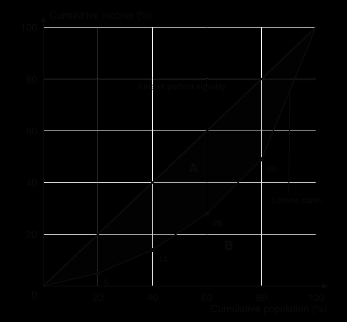
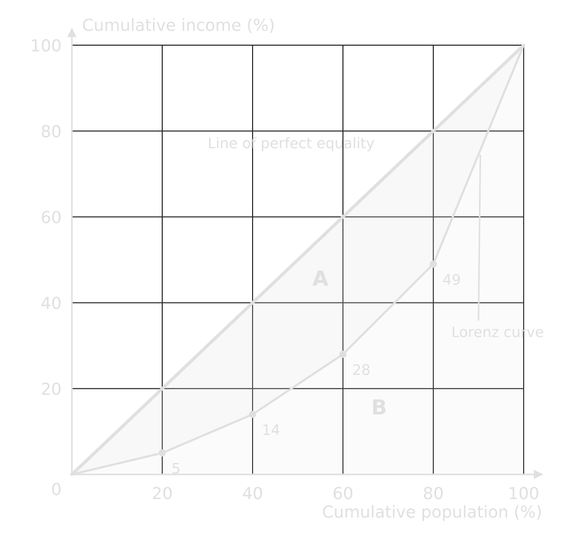
Lorenz curve for a hypothetical country: cumulative income 5, 14, 28, 49 and 100% at 20, 40, 60, 80 and 100% of population, below the line of perfect equality; area A between the line and curve, area B below the curve.Lorenz curve for a hypothetical country: cumulative income 5, 14, 28, 49 and 100% at 20, 40, 60, 80 and 100% of population, below the line of perfect equality; area A between the line and curve, area B below the curve.
The poorest 20% receive 5% of income and the richest 20% receive 51%. The curve bows well below the line of perfect equality; the shaded area A, as a share of A + B, is the Gini coefficient (here 0.42). Hypothetical data.

Worked example

In a country, the poorest fifth of households receive 5% of income, and the next four fifths receive 9%, 14%, 21% and 51%. Construct the Lorenz curve and determine the Gini coefficient.

Show the solution

Step 1: cumulative shares. 5, 5 + 9 = 14, 14 + 14 = 28, 28 + 21 = 49, 49 + 51 = 100%. Plot (20, 5), (40, 14), (60, 28), (80, 49) and (100, 100) and join them to (0, 0).

Step 2: area B under the curve. Treat each fifth as a trapezium of width 0.2 and average height (left + right) ÷ 2, using proportions:

B=0.2×(0+0.052+0.05+0.142+0.14+0.282+0.28+0.492+0.49+1.002)=0.292B=0.2×(20+0.05​+20.05+0.14​+20.14+0.28​+20.28+0.49​+20.49+1.00​)=0.292

Step 3: the Gini coefficient. G = 1 − 2B = 1 − 0.584 = 0.416, or about 42 on the 0–100 scale: a moderately high level of inequality.

Photographs, satellite images and field sketches

Photographs and satellite images are stimulus material in their own right. To describe a ground-level photograph, divide it into foreground, middle ground and background, and describe what is in each with its position ("in the left foreground, terraced fields on a steep slope"). For an aerial or satellite image, give the scale or approximate size, the orientation and the land uses or landforms visible, using compass directions.

A field sketch is a simplified drawing of a view made in the field. It shows only what is relevant to the investigation, with labels (names) and annotations (explanations), a title, the direction of view and the date. A field sketch can be better evidence than a photograph because it forces the geographer to select and interpret features rather than record everything.

Exam tip

Label and annotate are different command terms. A label names a feature in one or two words ("river cliff"); an annotation explains it in a short phrase ("river cliff: erosion on the outer bend, where velocity is highest"). Where a question says annotate, labels alone earn little credit.

Calculations that summarise data

Simple calculations turn raw data into figures that can be compared between places or over time. They appear in structured questions ("State the difference between…", "Estimate…", "Determine…") and throughout fieldwork. Show each step with its unit; a correct method with a slip in the arithmetic can still earn credit, while a bare wrong number earns nothing.

Averages and measures of spread

The three averages describe the typical value of a data set in different ways. The mean is the total divided by the number of values; it uses every value, so a single extreme value pulls it up or down. The median is the middle value when the data are in order, and is not affected by extremes. The mode is the most frequent value, useful for categories ("the modal shop type is a café").

xˉ=∑xnxˉ=n∑x​

Measures of spread show how far the values vary. The range is the largest value minus the smallest. The interquartile range is the upper quartile minus the lower quartile: the spread of the middle half of the data, which ignores the extremes. Two sites with the same mean can have very different spreads, so a description of data gives both an average and a measure of spread.

Worked example

A pedestrian count at eleven sites in a town centre recorded, over ten minutes each: 12, 18, 25, 25, 31, 36, 44, 52, 67, 88 and 214 people (hypothetical data). Determine the mean, median, mode, range and interquartile range, and suggest which average best describes a typical site.

Show the solution

Step 1: total and mean. Σx = 612; mean = 612 ÷ 11 = 55.6 people.

Step 2: median. The data are already in order; the 6th of 11 values is 36 people.

Step 3: mode. 25 appears twice: mode = 25 people.

Step 4: range. 214 − 12 = 202 people.

Step 5: interquartile range. The lower quartile is the median of the five values below the median (12, 18, 25, 25, 31) = 25; the upper quartile is the median of the five above it (44, 52, 67, 88, 214) = 67. IQR = 67 − 25 = 42 people.

Step 6: interpret. The site with 214 people (probably at the main shopping street) is an anomaly that pulls the mean up to 55.6, higher than eight of the eleven counts. The median (36) and the IQR (42) describe a typical site better. Without the anomaly the mean would be 39.8.

Percentages and percentage change

A percentage expresses a part as a share of 100, which allows places of different size to be compared. Percentage change compares a new value with the original one, and is always divided by the original value.

Percentage change=new value−original valueoriginal value×100Percentage change=original valuenew value−original value​×100

Worked example

International tourist arrivals in a region rose from 1.25 million in 2015 to 1.6 million in 2023, while hotel occupancy in one resort fell from 240 rooms a night to 180. Determine the percentage change in each.

Show the solution

Arrivals: (1.6 − 1.25) ÷ 1.25 × 100 = 0.35 ÷ 1.25 × 100 = +28%.

Occupancy: (180 − 240) ÷ 240 × 100 = −60 ÷ 240 × 100 = −25%.

Percentages of percentages need care: a fall from 20% to 15% unemployment is a fall of 5 percentage points, but a percentage change of −25%. A fall of 25% followed by a rise of 25% does not return to the start (240 → 180 → 225).

Densities and ratios

A density is an amount per unit of area. Population density is the number of people per km²; drainage density is the total length of streams per km² of a drainage basin. Densities allow areas of different size to be compared, which is why they suit choropleth maps.

Population density=total populationarea (km2)Population density=area (km2)total population​

A ratio compares two quantities. The sex ratio is the number of males per 100 females (1,060 males to 1,000 females gives 106). The dependency ratio compares the population of dependent age with the population of working age.

Dependency ratio=population aged 0–14+population aged 65+population aged 15–64×100Dependency ratio=population aged 15–64population aged 0–14+population aged 65+​×100

Worked example

A country has 2.4 million people aged 0–14, 6.4 million aged 15–64 and 1.6 million aged 65 and over. Determine its dependency ratio, and its youth and old-age dependency ratios.

Show the solution

Total: (2.4 + 1.6) ÷ 6.4 × 100 = 4.0 ÷ 6.4 × 100 = 62.5 dependants per 100 people of working age.

Youth: 2.4 ÷ 6.4 × 100 = 37.5. Old age: 1.6 ÷ 6.4 × 100 = 25.0.

The ratio assumes that everyone aged 15–64 works and no one outside that range does; in reality many 15–19-year-olds are in education and many people over 65 work, so the measure is an approximation.

Measuring concentration and dispersion

Two measures describe how features are spread across space. The nearest neighbour index (RnRn​) describes the pattern of points on a map; the location quotient describes whether an activity is concentrated in one area compared with a larger region.

Rn=2dˉnARn​=2dˉAn​​

Here dˉdˉ is the mean distance from each point to its nearest neighbour, n the number of points and A the area, in matching units (km and km²). Rn=0Rn​=0 means all points are clustered at one place, about 1 means a random pattern, and 2.15 means a perfectly regular (uniform) pattern, as in a triangular grid.
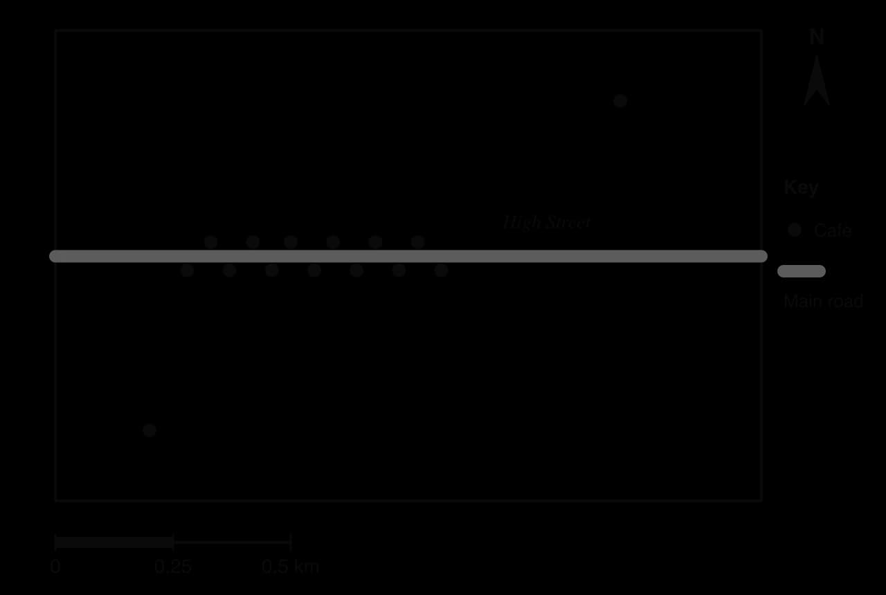
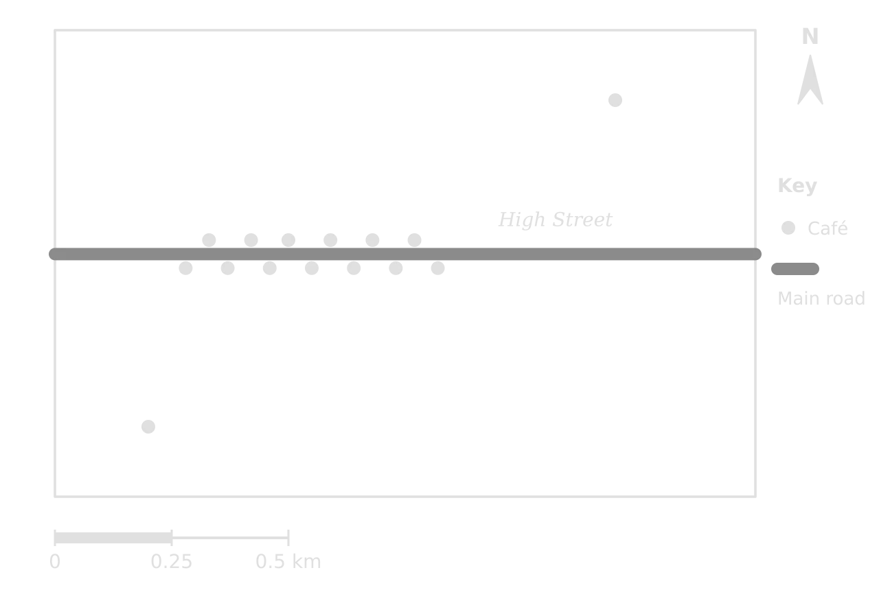
Dot map of 15 cafés in a hypothetical 1.5 km by 1.0 km area: 13 lie close together on both sides of the High Street, one is in the north-east and one in the south-west; scale bar 0.5 km.Dot map of 15 cafés in a hypothetical 1.5 km by 1.0 km area: 13 lie close together on both sides of the High Street, one is in the north-east and one in the south-west; scale bar 0.5 km.
Thirteen of the fifteen cafés line both sides of the High Street, 70–80 m from their nearest neighbour; the other two are isolated, 350 m and 520 m from the nearest café. Hypothetical data.

Worked example

The dot map shows 15 cafés in an area of 1.5 km². Measured on the map, the nearest-neighbour distances are 80, 70, 70, 70, 70, 70, 70, 70, 70, 70, 70, 70, 80, 520 and 350 m. Determine the nearest neighbour index and describe the pattern it shows.

Show the solution

Step 1: mean distance. Σd = 1,800 m; d̄ = 1,800 ÷ 15 = 120 m = 0.12 km (use km to match the area in km²).

Step 2: density term. n ÷ A = 15 ÷ 1.5 = 10; √10 = 3.162.

Rn=2×0.12×3.162=0.76Rn​=2×0.12×3.162=0.76

Step 3: interpret. 0.76 lies between clustered (0) and random (1), so the pattern tends towards clustering, which matches the line of cafés along the High Street.

Step 4: the effect of the boundary. If the same 15 cafés were measured within a study area of 3.0 km², R_n = 2 × 0.12 × √5 = 0.54, apparently more clustered. The index depends on the area chosen, so the boundary must be justified and kept the same when places are compared. The index also cannot recognise a linear cluster as a cluster in its own right.

The location quotient compares an activity’s share of the total in an area with its share in a larger reference area, usually the country. It is most often calculated for employment.

LQ=ei/eEi/ELQ=Ei​/Eei​/e​

Here eiei​ is employment in activity i in the area and ee is total employment in the area; EiEi​ and EE are the same figures for the reference area. LQ > 1 means the activity is more concentrated in the area than in the country, LQ < 1 that it is under-represented, and LQ = 1 that its share is the same.

District

Tourism jobs

All jobs

Share in tourism

Location quotient

X (coastal resort)

1,800

12,000

0.15

0.15 ÷ 0.04 = 3.75

Y (industrial city)

900

30,000

0.03

0.03 ÷ 0.04 = 0.75

Z (market town)

400

10,000

0.04

0.04 ÷ 0.04 = 1.00

Country (reference)

60,000

1,500,000

0.04

1.00

Worked example

Using the table of hypothetical employment data, determine the location quotient for tourism in district X, and classify districts X, Y and Z by how concentrated tourism is in each.

Show the solution

Step 1: the national share. 60,000 ÷ 1,500,000 = 0.04 (4% of all jobs).

Step 2: the district share. In X, 1,800 ÷ 12,000 = 0.15 (15%).

LQX=0.150.04=3.75LQX​=0.040.15​=3.75

Step 3: classify. X (3.75): tourism is strongly concentrated, almost four times the national share. Z (1.00): the same share as the country. Y (0.75): under-represented. A location quotient shows relative specialisation, not size: Y has half as many tourism jobs as X but a much lower quotient because its economy is far larger.

Testing relationships and differences

Two statistical tests are used most in fieldwork, and their results can appear in a stimulus to be interpreted. Spearman’s rank correlation coefficient (rsrs​) measures the strength and direction of the relationship between two variables measured at the same sites, from +1 (perfect positive) through 0 (none) to −1 (perfect negative). Each variable is ranked (1 = highest; tied values share the mean of their ranks) and d is the difference between the two ranks of each pair.

rs=1−6∑d2n(n2−1)rs​=1−n(n2−1)6∑d2​

The value is then compared with a critical value for the number of pairs, n, at a chosen significance level, usually 0.05 (95% confidence) or 0.01 (99% confidence). If the value, ignoring its sign, is at least the critical value, the null hypothesis of no relationship is rejected. The chi-squared test does the same job for counts in categories, comparing observed frequencies (O) with those expected (E) if there were no difference.

χ2=∑(O−E)2EE=row total×column totalgrand totaldf=(r−1)(c−1)χ2=∑E(O−E)2​E=grand totalrow total×column total​df=(r−1)(c−1)

Worked example

(a) A student finds rsrs​ = 0.71 between distance from a city centre and environmental quality at 10 sites. The two-tailed critical values for n = 10 are 0.648 (0.05) and 0.794 (0.01). State what the result shows. (b) Of 40 shoppers questioned at an out-of-town retail park, 30 arrived by car and 10 by other means; of 40 in the town centre, 15 arrived by car and 25 by other means (hypothetical data). Determine χ² and state whether the difference is significant (critical values for df = 1: 3.84 at 0.05, 6.63 at 0.01).

Show the solution

(a) 0.71 is above 0.648 but below 0.794, so there is a strong positive correlation that is significant at the 0.05 level but not at the 0.01 level: the null hypothesis is rejected with 95% confidence.

(b) Step 1: expected values. Row totals are 40 and 40, column totals 45 (car) and 35 (other), grand total 80. E(car) = 40 × 45 ÷ 80 = 22.5 at each place; E(other) = 40 × 35 ÷ 80 = 17.5.

Step 2: χ². (30 − 22.5)² ÷ 22.5 = 2.50; (10 − 17.5)² ÷ 17.5 = 3.21; (15 − 22.5)² ÷ 22.5 = 2.50; (25 − 17.5)² ÷ 17.5 = 3.21. χ² = 11.43.

Step 3: interpret. df = (2 − 1)(2 − 1) = 1. 11.43 exceeds 6.63, so the difference in car use between the two places is significant at the 0.01 level.

Tip

A statistic needs three things to be complete: its value, the critical value it is compared with (for the right n or degrees of freedom), and the decision about the null hypothesis at a stated significance level.

Describing patterns, trends and anomalies

Many questions begin with "Describe…" a map, graph or table. A description says what the figure shows, not why. The most reliable structure is TEA: the Trend or general pattern, Evidence with figures and units from the stimulus, and the Anomaly or exception.

Step

For a graph or table

For a map

Trend or general pattern

The overall direction: rising, falling, fluctuating, peaking; strong or weak relationship

Where values are high and low, using compass directions and named places; clustered, linear, even or random

Evidence

Figures at the start, end, peak and turning points, with units and dates

Values or classes for named areas; distances; latitudes

Anomaly

A value that breaks the trend, quantified

A place that does not fit the pattern, located and quantified

Useful vocabulary makes descriptions precise: "increased steadily", "rose sharply after 1990", "fluctuated between", "peaked at", "a strong negative relationship", "concentrated in the north-east", "a linear pattern along the coast", "evenly spaced". Avoid vague words such as "a lot", "big" or "goes up and down" without figures.

Worked example

[2 marks] Describe the pattern of night-time air temperature shown on the isoline map of the city.

Show a model answer

Temperatures are highest in the CBD, at 18.4 °C, and decrease outwards in all directions ✓ to between 13.3 °C and 13.8 °C at the rural stations, a difference of about 5 °C ✓. An exception is the park north-east of the CBD, which is cooler (13.5 °C) than the built-up area around it ✓.

Three valid quantified points for 2 marks. An answer that only says "it is hotter in the centre" has no figures and would earn 1 mark at most.

Exam tip

In a "describe" question, quantifying is what moves an answer from one mark to two. Quote at least two figures from the stimulus, with units, and the place or date they refer to. Don’t explain unless asked: reasons earn nothing in a describe question and use up time.

Common mistake

Describing every bar or every area in turn ("A is 38, B is 72, C is 145…"). A description generalises first and then supports the generalisation with selected figures, instead of listing every value.

Evaluating sources

Geographers use maps, statistics, photographs, reports, news articles and interviews made by other people, and each has to be judged before it is trusted. Three questions apply to any source: is it accurate, is it relevant to the question, and is it free from bias?

Criterion

Questions to ask

Example

Accuracy

How were the data collected, by whom, with what sample and how recently? Are figures estimates?

A census every ten years is accurate for its year but dated by the next; informal settlements are often undercounted

Relevance

Does it cover the right place, scale and time? Does it measure the variable the question is about?

National GNI per capita says little about income in one rural province

Bias

Who produced it and why? Is anything left out? Is the language or framing one-sided?

A developer’s report on a new resort and a campaign group’s leaflet against it select different evidence

Representation

Do the map’s classes, the graph’s axes or the photo’s framing exaggerate a pattern?

A y-axis that starts at 90% makes a small fall look dramatic

A photograph shows one view at one moment, chosen by the photographer; an interview gives one person’s perception, which is valid evidence of that perception but not of the facts. Opinions, values and perceptions are legitimate geographical data when they are identified as such and compared with measured evidence.

Statistics can look objective and still reflect choices. Unemployment, poverty and even population totals depend on definitions (who counts as unemployed or poor), on how a sample was drawn, and on what governments choose to publish. Checking how a figure was defined and collected is therefore part of interpreting it.

Add to your notes: a one-page skills sheet with a small sketch of each map and graph type, one line on when to use it, and the formulas for percentage change, density, the dependency ratio, the nearest neighbour index, the location quotient and the Gini coefficient, each with a worked number.

Exam practice

Skills are tested in every paper, but most directly in the structured questions on Paper 1 options, where a topographic map extract is a common stimulus, and in Paper 2 Sections A and B. This structured question follows the Paper 1 format and uses the Ashby map extract.

Worked example

Using the topographic map extract of Ashby (scale 1:25,000, contour interval 10 m):

(a)(i) State the six-figure grid reference of the spot height in the south-east of the map. [1]

(a)(ii) Estimate the height of the land at the church at 343527. [1]

(b) Outline one advantage of the site of Ashby for a settlement. [2]

(c) Explain two ways in which the relief shown on the map could increase the risk of flooding in Ashby. [3+3]

Show the markscheme and model answers

(a)(i) 359514 ✓ (accept 358514–360515).

(a)(ii) About 45 m ✓: the church lies between the 40 m and 50 m contours (accept 41–49 m).

(b) The village is built at a crossing point of the River Lune ✓, where the road bridges the river, so routes from the north and south meet there, which helps trade and access ✓. (Alternative: flat land on the valley floor ✓ that is easy to build on and close to water ✓.)

(c) First way: the hill to the north-east of Ashby has very steep slopes, shown by closely spaced contours (a fall of about 85 m in the first 1 km south of the summit) ✓. Rain falling on steep slopes runs off quickly as overland flow instead of infiltrating ✓, so water reaches the river within a short time and raises its peak discharge as it passes the village ✓.

Second way: Ashby is built on the valley floor beside the river, its lowest buildings only a few metres above the channel (the church at about 45 m, the river at about 40 m) ✓. All the water from the surrounding slopes drains towards this lowest land ✓, so when the river overtops its banks the village is the first area to be flooded, especially the buildings closest to the channel ✓.

Each part of (c) earns 1 mark for the way and 2 for its development; using evidence from the map (contour spacing, heights) is what secures the development marks.

Exam tip

When a question says "using the map" or "using the graph", the evidence must come from the figure: name grid squares, quote heights, read values. A general answer that could be written without the stimulus is capped, however well it is explained.

Worked example

[2 marks] Suggest why a proportional symbol map is more suitable than a choropleth map for showing the number of tourist arrivals in each town on an island.

Show a model answer

Tourist arrivals are absolute numbers for points (towns), not rates for areas ✓. A choropleth map would shade whole districts as if visitors were spread evenly across them, and large districts would look important because of their size, while proportional circles show each town’s total directly at its location ✓.

Skills checklist

  • To do:

    I can give four- and six-figure grid references, directions, bearings and distances from a map, and convert between map and ground distances at 1:25,000 and 1:50,000.

  • To do:

    I can read relief from contours and spot heights, determine a gradient and draw a labelled cross-section with its vertical exaggeration.

  • To do:

    I can choose, read and construct choropleth, isoline, proportional symbol, dot and flow-line maps, and explain why each suits its data.

  • To do:

    I can read and construct line, bar, compound bar, scatter, triangular, logarithmic, rose and bipolar graphs.

  • To do:

    I can describe population pyramids and development diamonds, and construct a Lorenz curve and determine a Gini coefficient.

  • To do:

    I can determine the mean, median, mode, range, interquartile range, percentage change, densities and ratios, with units.

  • To do:

    I can determine and interpret a nearest neighbour index and a location quotient.

  • To do:

    I can describe a pattern or trend with figures and an anomaly, and evaluate a source for accuracy, relevance and bias.

Keep your place

In Augment the notes remember where you stopped and which pages you have finished.

Open in Augment

More IB Geography notes

  • Paper 3: the HL extensionThe page before this. HL only.
  • Planning fieldwork and the fieldwork questionThe next page.
  • Geography assessmentEach Geography paper, the internal assessment and grade boundaries.
  • IB GeographyThe Geography syllabus, how it is assessed and every notes page.

Carry on with Geography in Augment

With a free account, Augment remembers where you stopped in the notes and which questions you have marked.

Start free