Collecting and processing data
Record raw data precisely, handle uncertainties, errors and outliers, choose the right statistical test for your design and present results in clear graphs with error bars, using one worked investigation throughout.
- IB Sports, Exercise and Health Science
- Internal assessment
- SL and HL
Data collection turns the plan into numbers; processing turns the numbers into evidence that can answer the research question. Both are assessed mainly by the data analysis criterion, which rewards recording and processing that are clear (a reader can follow what was done) and precise (correct units, decimal places, significant figures and graph conventions), with appropriate attention to uncertainties.
The worked investigation from "Planning the scientific investigation" continues here: twelve students completed countermovement jumps after 0, 5, 10 and 15 min of dynamic warm-up, in a counterbalanced cross-over design. All its data are hypothetical. The statistics used are explained in full, with the formulae, in "Data analysis, statistics and the data booklet"; here they are applied to the decisions made in one investigation.
Quantitative and qualitative data
The analysis rests on quantitative data, but qualitative data are what make the numbers interpretable. A jump height of 24.3 cm means little on its own; "P07, 5 min, jump 2: right foot slipped at take-off" explains it and justifies what is done with it. Qualitative observations also supply the specific weaknesses that the evaluation needs, and they show the moderator that the data collection was closely observed.
Useful qualitative observations in SEHS include technique faults and changes in technique across trials, comments about fatigue, soreness, boredom or nervousness, distractions (another class entering the hall), equipment problems, and environmental conditions such as temperature or wind for outdoor work. Record them at the time, next to the measurement they affect, in a column of the raw data table or a dated log.
Session | Participant | Observation |
|---|---|---|
2 | P04 | Bent knees on landing in jump 1; jump repeated (repeat recorded) |
2 | P07 | Right foot slipped at take-off, jump 2 of the 5 min condition |
3 | P11 | Reported mild calf soreness from a football match two days earlier |
3 | All | Hall temperature 19 °C (lowest of all sessions) |
4 | P05 | Said they felt "tired from the jog" after the 15 min warm-up |
Running the data collection
Consistency is the aim of every session. The same tester gives the same scripted instructions, the equipment is set up in the same place and checked at the start, and the control variables are confirmed and recorded before any measurement. Small departures are inevitable in a school; what matters is that they are noticed, written down and dealt with in a way the report can explain.
Problems that arise during collection are part of the investigation, not something to hide. A participant who is ill on a test day, a flat battery in the heart rate monitor, a fire drill in the middle of a session: each needs a decision (reschedule, repeat, exclude) and a record of it. Making that decision consistently, by a rule set in advance where possible, keeps the data fair.
Recording raw data
Raw data are the values exactly as measured, before any calculation. Record them directly into a prepared table (on paper or in a spreadsheet) during the session, never from memory afterwards, and keep the original even after processing. The report usually shows a sample of the raw data, or all of it in an appendix if it is long, so that the reader can see how processed values were obtained.
A clear title saying what the table shows.
Column headings with the quantity, the unit and the uncertainty: "Jump height / cm ± 0.1 cm". Units go in the heading, not after every number.
Every value given to the same number of decimal places, matching the resolution of the instrument (a mat that reads to 0.1 cm gives 31.0, not 31).
Participant codes, never names.
A column or footnote for qualitative observations next to the values they concern.
Participant | 0 min: jump 1 / cm | Jump 2 / cm | Jump 3 / cm | 10 min: jump 1 / cm | Jump 2 / cm | Jump 3 / cm |
|---|---|---|---|---|---|---|
P01 | 28.2 | 27.6 | 27.5 | 30.4 | 30.9 | 30.3 |
P02 | 42.0 | 42.0 | 40.2 | 45.1 | 44.8 | 45.3 |
P03 | 31.9 | 30.9 | 31.5 | 32.3 | 32.9 | 32.6 |
P04 | 36.3 | 37.1 | 37.2 | 38.9 | 40.2 | 40.4 |
The table is an extract (hypothetical data): the full raw data set has 12 participants × 4 conditions × 3 jumps = 144 values, plus heart rates and room temperatures. Each height is recorded to 0.1 cm with an uncertainty of ±0.1 cm, the resolution of the mat.
Accuracy, precision and errors
Two words describe the quality of measurements, and they are often confused.
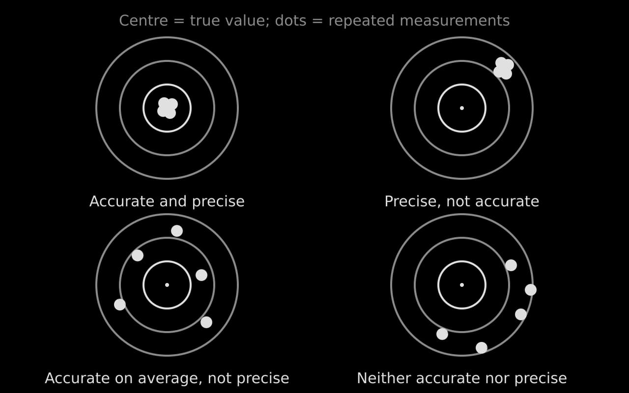
Accuracy and precision are linked to two kinds of error. Random errors scatter values unpredictably above and below the true value and reduce precision; systematic errors shift every value in the same direction and reduce accuracy.
Source of error in SEHS | Type | How to reduce it |
|---|---|---|
Hand-timing with a stopwatch (reaction time at start and stop) | Random, and systematic if the timer always reacts late | Timing gates, or video at a known frame rate |
Participant’s effort varies between trials | Random | Repeats; scripted encouragement; adequate rest |
Heart rate monitor strap loose | Random (dropouts and spikes) | Moisten and fit the strap; check the reading at rest |
Scales that read 0.5 kg high | Systematic | Calibrate with a known mass; correct or zero the scale |
Landing with bent knees on a jump mat | Systematic (heights too high) | Standardised landing instruction; observe every landing |
Parallax when reading a video frame at an angle | Systematic | Camera perpendicular to the plane of motion, with a scale in view |
Learning across sessions (order effect) | Systematic for whichever condition comes last | Familiarisation session; counterbalanced order |
The distinction matters in the evaluation. A random error affects how confident you can be in a mean, and more repeats would help. A systematic error affects whether the values are correct at all, and more repeats of the same flawed procedure would not help. A systematic error that affects all conditions equally (a mat that reads 1 cm high for everyone) does not change a comparison between conditions, but it does matter when values are compared with published norms.
Uncertainties
Every measurement has an uncertainty: the range within which the true value probably lies. Stating uncertainties, carrying them through calculations and judging their effect on the conclusion is one of the three strands of the data analysis criterion, and the conclusion criterion asks you to interpret the processed data "including associated uncertainties".
Uncertainty of a single measurement
Digital instruments: plus or minus the smallest reading (a mat that reads to 0.1 cm: ±0.1 cm; a heart rate monitor: ±1 beat min⁻¹).
Analogue scales: plus or minus half the smallest division (a tape measure marked in millimetres: ±0.5 mm), larger if the reading is difficult.
Human-operated timing: the instrument’s resolution (0.01 s) understates the real uncertainty, which is dominated by reaction time (often ±0.1–0.2 s). State the larger value and explain it.
Uncertainty from repeated measurements
When the same thing is measured several times, the spread of the readings is usually larger than the instrument uncertainty, and it is the better estimate. A simple, accepted method is half the range of the repeats: for P02’s three jumps with no warm-up (42.0, 42.0 and 40.2 cm), the mean is 41.4 cm and the uncertainty is (42.0 − 40.2) ÷ 2 = ±0.9 cm. For a group of participants, the standard deviation describes the spread around the group mean.
The comparison between the two kinds of uncertainty is worth making in the report. Here the mat’s ±0.1 cm is small compared with the ±0.9 cm variation between one person’s jumps, so the main source of uncertainty is the participant, not the instrument. That tells you where an improvement should be aimed.
Propagating uncertainties
When a value is calculated from measured quantities, their uncertainties combine. The data booklet gives the rules: for a sum or difference, absolute uncertainties add; for a product or quotient, fractional (percentage) uncertainties add; for a power, the fractional uncertainty is multiplied by the power.
Outliers
An outlier is either a genuine, if unusual, result or the product of a mistake. Only the second kind should be removed, and only with a reason that comes from the investigation itself, not from the fact that the value spoils a trend. That is why qualitative observations matter: they are usually the evidence that justifies the decision. A statistical rule for outliers is not needed: a clear explanation based on what happened is enough.
Processing the data
Processing means turning raw values into the quantities that answer the research question: means for each participant and condition, then a summary for each condition, then a comparison. Show one example of each type of calculation, with the formula and the working, then present the results of the others in a table. Spreadsheets are encouraged; say which function was used for a statistical test.
Participant means
Each participant’s three jumps in a condition were averaged (the mean), giving one value per participant per condition. Using the mean of three rather than the best of three reduces the effect of random variation; the best jump is also a defensible choice for a maximal test, as long as the report says which was used and why.
Participant | 0 min / cm | 5 min / cm | 10 min / cm | 15 min / cm |
|---|---|---|---|---|
P01 | 27.8 | 29.2 | 30.5 | 29.5 |
P02 | 41.4 | 42.7 | 45.1 | 44.5 |
P03 | 31.4 | 31.2 | 32.6 | 31.7 |
P04 | 36.9 | 39.0 | 39.8 | 39.9 |
P05 | 25.6 | 26.1 | 25.8 | 25.3 |
P06 | 37.6 | 40.0 | 39.1 | 39.8 |
P07 | 33.6 | 36.3* | 36.9 | 36.3 |
P08 | 29.4 | 31.2 | 31.8 | 31.9 |
P09 | 44.3 | 45.6 | 45.5 | 46.1 |
P10 | 31.6 | 33.5 | 33.6 | 33.4 |
P11 | 27.0 | 28.9 | 29.7 | 29.7 |
P12 | 35.1 | 35.5 | 36.0 | 35.3 |
Mean countermovement jump height (cm) of each participant’s three jumps in each condition (hypothetical data). *Mean of two jumps: the second was excluded because of a recorded slip. Uncertainty of each individual jump ±0.1 cm.
Summarising each condition
For each condition, the mean of the 12 participant means estimates the group’s typical jump height, and the standard deviation (SD) describes how much participants differ from it. The standard error (SD ÷ √n) estimates how precisely the group mean is known.
Warm-up duration / min | Mean jump height / cm | SD / cm | Standard error / cm | Mean heart rate before jumps / beats min⁻¹ |
|---|---|---|---|---|
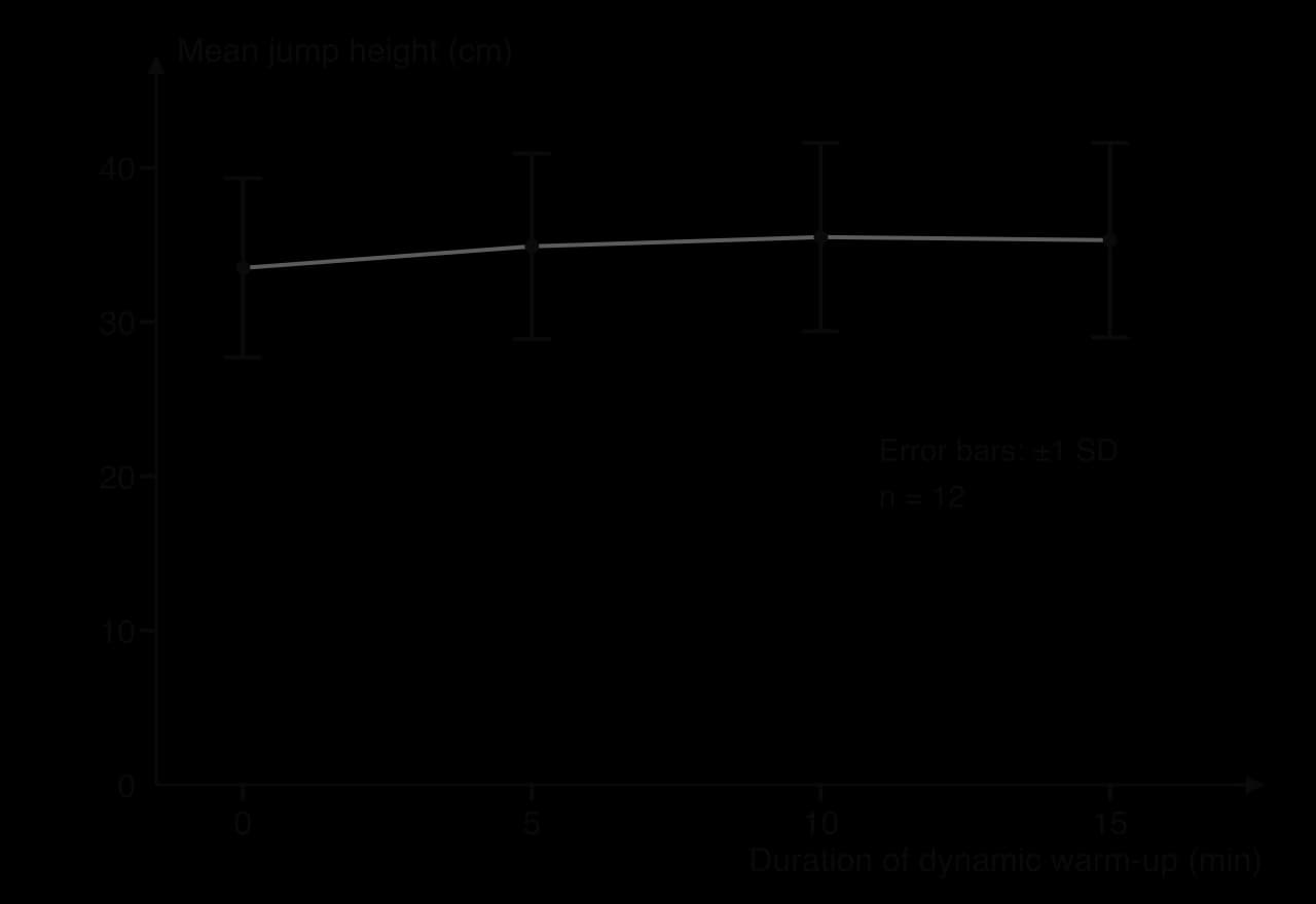
0 | 33.5 | 5.8 | 1.7 | 78 |
5 | 34.9 | 6.0 | 1.7 | 102 |
10 | 35.5 | 6.1 | 1.7 | 109 |
15 | 35.3 | 6.3 | 1.8 | 113 |
Summary for 12 participants (hypothetical data). Heart rate was measured at the end of the 2 min rest and confirms that the four conditions differed physiologically.
Two things stand out. The mean rises by 1.4 cm from 0 to 5 min and by a further 0.6 cm to 10 min, then falls slightly at 15 min, the shape the hypothesis predicted. But the SD in every condition (about 6 cm) is about three times larger than the whole change in the mean (2.0 cm): participants differ from each other far more than any one participant changes between conditions.
Processed values follow the same conventions as raw ones. Means are usually given to the same number of decimal places as the raw data, or one more when many values are averaged, and SDs and standard errors to the same decimal place as the mean they describe. Percentages and test statistics are rounded to a sensible number of significant figures (two or three); a p-value is given to two significant figures or as "p < 0.001".
Choosing a statistical test
A statistical test answers one question: could a difference or relationship this large have arisen by chance, if there were really none? The choice of test follows from the research question and the design, so decide it at the planning stage, not after seeing the data.
Research question asks about | Design | Analysis |
|---|---|---|
A difference between two conditions, same participants | Cross-over (repeated measures) | Paired t-test on each participant’s two values |
A difference between two separate groups | Independent groups | Unpaired (independent) t-test |
A trend across several levels of the IV | Four or more levels | Means with error bars on a line graph; trend line with R²; t-tests between the key pairs chosen in advance |
A relationship between two measured variables | Correlational | Scatter graph; correlation coefficient r compared with the critical value for n; R² |
The t-test compares two means, taking account of the spread and the sample size. The p-value it gives is the probability of a difference at least as large as the one observed if the null hypothesis were true. If p < 0.05, the difference is called statistically significant, the null hypothesis is rejected and the alternative hypothesis is supported. A spreadsheet calculates it directly: in most spreadsheets, T.TEST(range1, range2, 2, 1) gives a two-tailed paired test and T.TEST(range1, range2, 2, 2) an unpaired one. A two-tailed test is the usual choice, even when H₁ predicts a direction.
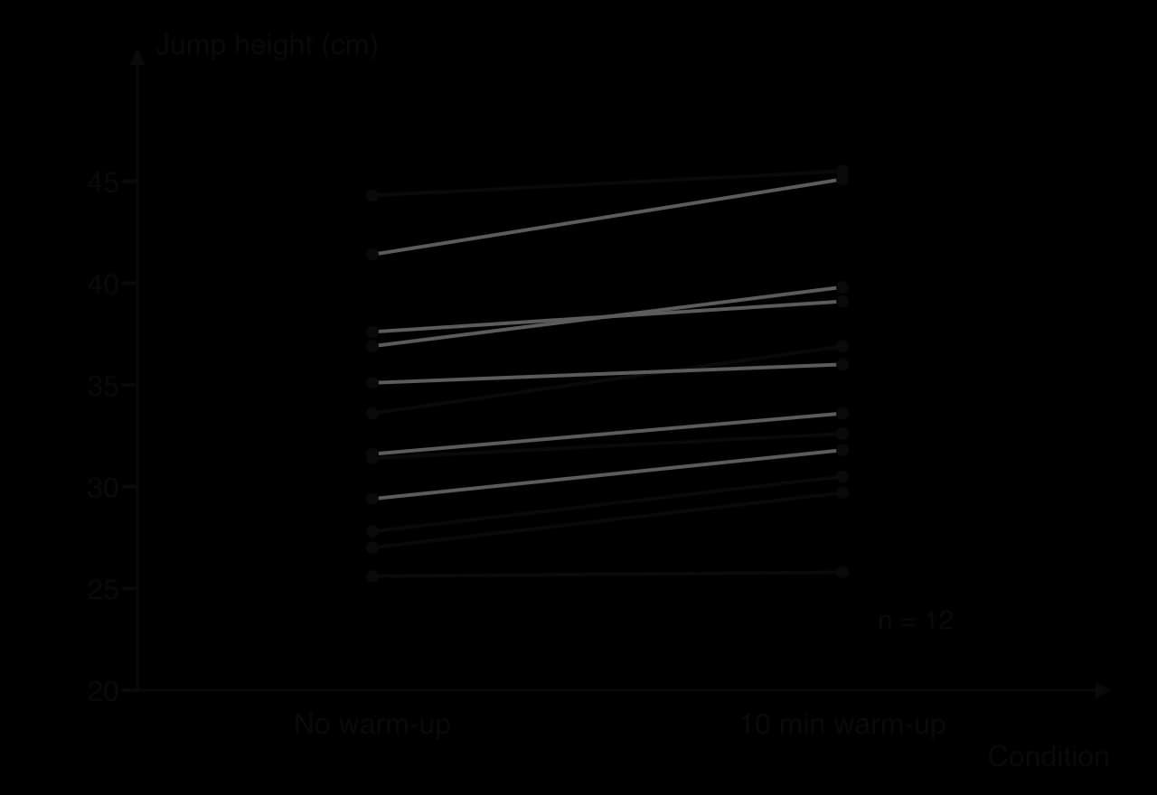
The other planned comparisons complete the picture. Paired t-tests give a mean difference of 1.5 cm from 0 to 5 min (p = 0.00011), 0.6 cm from 5 to 10 min (p = 0.035) and −0.25 cm from 10 to 15 min (p = 0.15, not significant). Running several tests on the same data raises the chance that one is significant by luck, so a careful report says how many tests were run, treats a result such as p = 0.035 with caution and bases its main conclusion on the comparison planned in the hypotheses.
Correlational designs
When both variables are measured rather than manipulated, the relationship is tested with the correlation coefficient r. A value of r near +1 or −1 shows a strong linear relationship; near 0, none. Compare |r| with the critical value for your sample size at p = 0.05 (from a table): if |r| is larger, the correlation is significant. The coefficient of determination R² gives the proportion of the variation in one variable that is accounted for by the line of best fit.
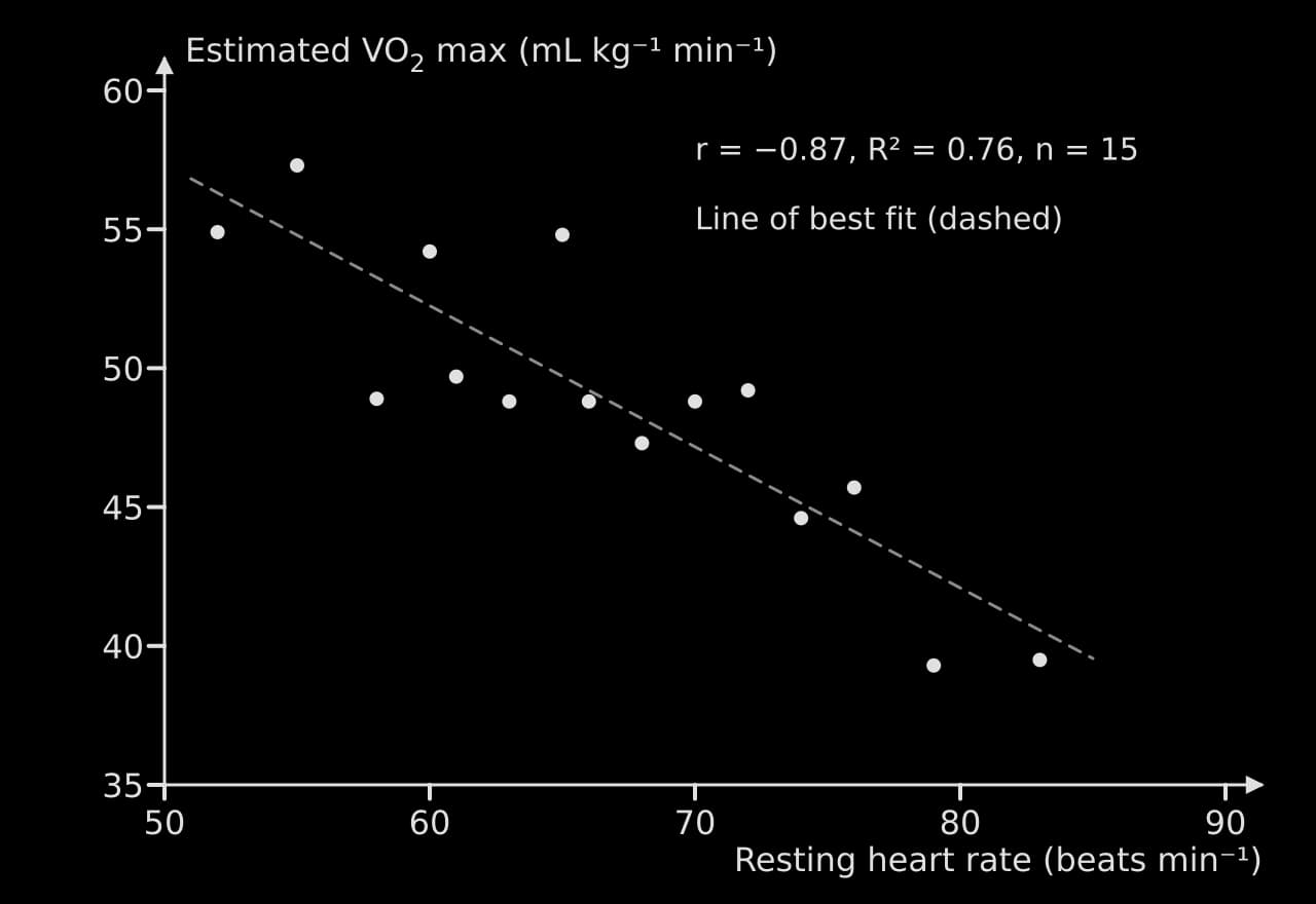
Even a significant correlation does not show causation. Students with a low resting heart rate may have a higher estimated VO₂ max because both result from endurance training, a third variable. The conclusion of a correlational study says that the variables are associated, and suggests mechanisms, but does not claim that one causes the other.
Presenting the data in graphs
A graph should let the reader see the answer to the research question at a glance, so its type follows the variables. A continuous independent variable (duration, step height, pressure) is plotted on a line or scatter graph with a scaled x-axis. A categorical independent variable (music or no music, blocked or random practice) uses a bar or column chart. Two measured variables use a scatter graph with a line of best fit. Pie charts and 3-D effects rarely help.
A title or caption that states what is plotted, the sample size and what the error bars show.
Both axes labelled with the quantity and unit: "Mean jump height (cm)".
Scales that use the space and increase evenly; start the y-axis at zero for bar charts, and mark any break clearly.
Points for means, with error bars for the spread or uncertainty.
A line of best fit or a smooth curve only where the trend is justified; joining points with straight lines is acceptable for a few discrete levels.
What error bars show
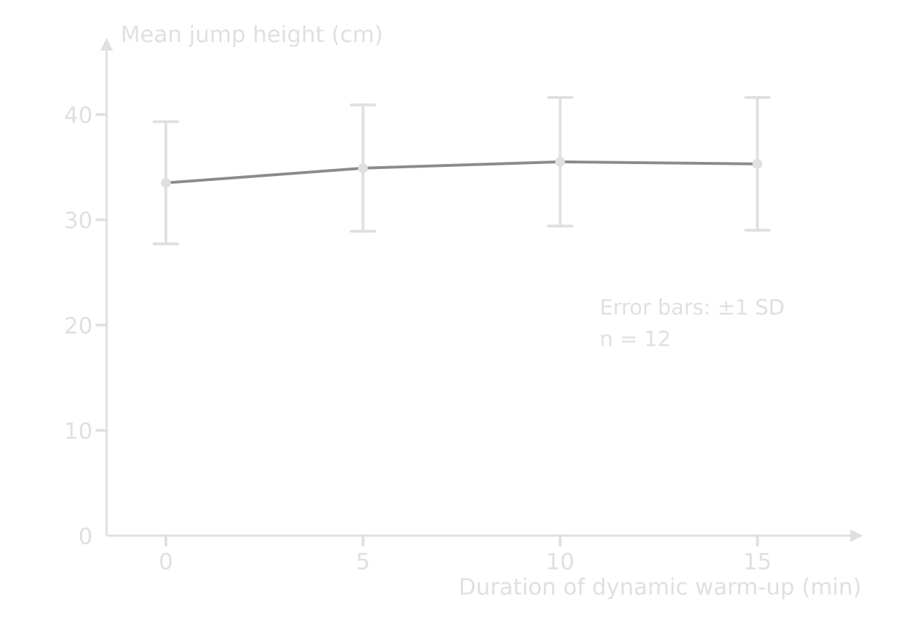
Error bars can show the standard deviation, the standard error, the range or a measurement uncertainty, and each says something different, so the caption must say which is used. SD bars show how much individuals vary; SE bars show how precisely the mean is known and are √n times shorter (about 3.5 times for n = 12); range bars show the extremes. As a rough rule for independent groups, if SD bars overlap heavily the difference is unlikely to be significant, and if they do not overlap at all it probably is. The t-test, not the bars, makes the decision.
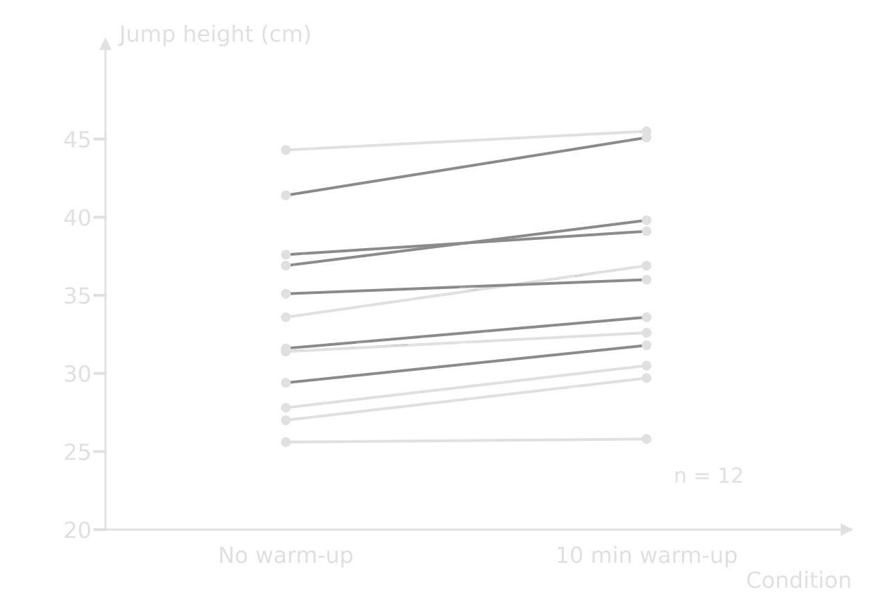
That rough rule fails for a cross-over design, as the warm-up data show. The SD bars overlap almost completely, yet the paired test is highly significant, because every participant improved. A second graph that shows each participant’s change makes the paired result visible.
Trend lines, interpolation and extrapolation
A trend line summarises a relationship, and R² shows how well it fits. With only four levels of the independent variable, as in the warm-up investigation, a curved trend line of high order can pass through every point (R² close to 1) while saying nothing reliable about the shape. Choose the simplest line or curve that theory supports, and say why.
Reading a value between measured levels (interpolation) is reasonable if the trend is smooth: a 7 min warm-up would probably give a mean between the 5 and 10 min values. Reading beyond the measured range (extrapolation) is risky, because the mechanism may change: the data contain no information about a 30 min warm-up, and fatigue could make it worse rather than better. The conclusion must stay within the range investigated.
Data from databases and simulations
A database investigation uses secondary data, and its research design is about selection rather than measurement. The report names the database, explains why it is trustworthy (who collected the data, how, when and with what definitions), states the criteria used to filter it (years, age groups, events, countries with complete data) and describes how the sample was drawn if not all records were used. These decisions are the database equivalent of controlling variables.
Check definitions: "physically inactive" or "obesity" may be defined differently across countries or years, which can create a spurious change.
Watch for missing data: countries or athletes with incomplete records may differ systematically from the rest, so say how gaps were handled.
Keep a record: download date, version and the exact filters, so the extraction can be repeated.
Uncertainty still applies: published values are rounded and often have confidence intervals; use them.
A spreadsheet model or simulation generates data from equations. The report states the equations and the assumptions behind them (no air resistance in a projectile model, for example), tests the model against at least a few real measurements, and treats the gap between model and reality as part of the evaluation.
Data collection and processing checklist
- To do:
Raw data are recorded during each session, with units and uncertainties in the headings and consistent decimal places.
- To do:
Participants are coded and qualitative observations are recorded next to the values they affect.
- To do:
I can name the main random and systematic errors in my method and say how I reduced them.
- To do:
I have stated the uncertainty of each instrument and compared it with the variation between repeats.
- To do:
Any uncertainty in a calculated value is propagated with the data booklet rules and rounded consistently.
- To do:
Every outlier is identified, and its inclusion or exclusion is justified by what happened at the time.
- To do:
One example of each calculation is shown with its formula, and the results are presented in a clear table.
- To do:
The statistical test matches the research question and the design (paired or unpaired, t-test or correlation), and its result is interpreted against p = 0.05.
- To do:
Each graph has a suitable type, labelled axes with units, sensible scales and error bars whose meaning is stated.
- To do:
For database or simulation data, the source, filters, sampling and assumptions are stated.
Carry on with SEHS in Augment
With a free account, Augment remembers where you stopped in the notes and which questions you have marked.