Paper 1B: data-based questions

What Paper 1B contains

Paper 1 has two parts that you sit together, without a break: Paper 1A (multiple-choice questions) and Paper 1B. Paper 1B is worth 25 marks at both SL and HL, so the same skills are tested at the same depth whichever level you take. It contains data-based questions and questions on experimental work. Each question gives you a short account of a study, usually invented or simplified for the paper, with its results in a table, a graph or both, and then asks a series of short parts about it.

The studies come from all three themes: exercise physiology and nutrition, biomechanics, and sports psychology and motor learning. You are not expected to have met the study before. The marks come from two sources: using the information in front of you accurately (reading values, describing trends, calculating, judging the evidence) and bringing in course knowledge to explain the results (a physiological mechanism, a law of motion, a theory of learning). The best answers do both in the same sentence.

Paper 1 gives you a little over a minute and a half per mark at both levels. Because 1A and 1B share the same time, you decide how to split it. At about one minute per multiple-choice question (roughly 30 minutes at SL and 40 at HL), about an hour is left for the 25 marks of 1B at either level, including a few minutes at the end to check calculations.

The command terms in 1B are the same as in the rest of the course, but here they point at the data. The table shows the ones you meet most often and what each one needs.

A typical question runs from the lower assessment objectives to the higher ones. It opens with one or two short "state" or "calculate" parts, moves to "describe" and "compare", and ends with "explain", "evaluate" or "suggest". Marks rise as the demand rises, so the last two or three parts of a question are often worth half its marks.

Reading a study before the questions

Read the whole stimulus once before you look at the first part. Most of the parts test whether you understood how the study was set up, and the answer to a later part (an evaluation or an improvement) is often hidden in a detail of the method. Reading the stimulus in a fixed order means nothing is missed.

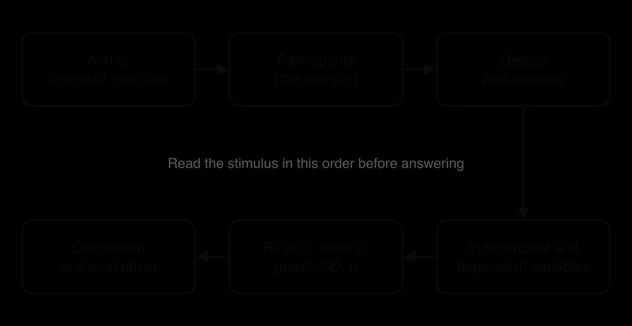
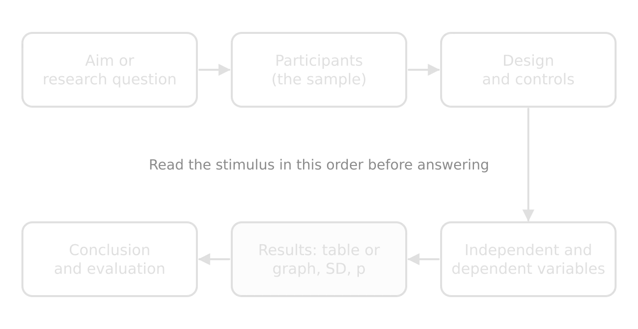
Underline or box each of these as you read. A minute spent marking up the method saves several minutes later, because the "evaluate" and "suggest" parts at the end of the question usually depend on details of the sample and the controls.

Aim, research question and hypothesis

The aim says what the researchers wanted to find out. A focused research question names both variables and the group studied: "What is the effect of fluid replacement on heart rate during 60 minutes of cycling in trained cyclists?" Some stimuli also give a hypothesis. The null hypothesis states that there is no effect or no relationship (fluid replacement has no effect on heart rate); the alternative hypothesis states that there is one. A statistical test decides whether the data allow the null hypothesis to be rejected.

Variables

The independent variable is the one the researchers change or select (the drink condition, the type of practice, the training programme). The dependent variable is the one they measure to see the effect (heart rate, jump distance, accuracy). Control variables are kept the same so that they cannot explain the difference: the exercise intensity, the room temperature, the time of day, the warm-up. A confounding variable is a factor that was not controlled and varies with the independent variable, so it offers an alternative explanation for the result.

Participants and the sample

Check how many participants there were, who they were (age, sex, training status, sport) and how they were chosen. Small samples (8–15 people are common in sport science) make results less reliable, because one or two unusual people can shift a mean. A sample of one kind of person, such as trained young men, limits how far the result can be applied to women, older adults, children or untrained exercisers. Random sampling from a population, or at least random allocation to groups, reduces the risk that the groups differ before the study starts.

Study designs

The design decides which comparisons are fair and which statistical test fits. The three you meet most often in Paper 1B are set out in the table.

Correlational studies are a fourth type: the researchers measure two variables in the same people without changing either (for example, approach speed and jump distance in a group of long jumpers). They can show whether two variables are related, but they cannot show that one causes the other.

Controls against bias

Researchers use several tools to stop expectations and chance from producing a result. A placebo is an inactive treatment that looks, tastes or feels like the real one, so that any effect of simply believing in a treatment (the placebo effect) is the same in both conditions. Blinding hides the condition from the participants (single-blind) or from both the participants and the researchers who measure the results (double-blind). Random allocation to groups or orders stops the researcher choosing who gets what. A familiarisation session before the real trials reduces learning effects on unfamiliar tests.

This short design is a cross-over design without a placebo, because music cannot be disguised. That is a limitation worth noting in an evaluation: the runners knew which condition they were in, and their beliefs about music could have affected their rating of perceived exertion, which is a self-reported measure.

Interpreting tables and graphs

Start with the axes, units and key

Before reading any value, read the axis labels, the units, the scale and the key. Three features catch students out in Paper 1B. First, an axis may not start at zero; a break symbol (two short diagonal lines) often shows this, and a shortened axis makes differences look larger than they are. Second, a graph may show means with error bars, and the caption says what the bars are (SD, SE or range). Third, a table may give "mean ± SD" in one cell, so "64.2 ± 5.1" means a mean of 64.2 with a standard deviation of 5.1.

Describing a trend

A good description has three parts: the overall direction of the trend, values with units at the start and end (or at key points), and any change in the pattern, such as a plateau, a peak or an exception. "Mean heart rate increased steadily from 139 beats min⁻¹ at 10 minutes to 164 beats min⁻¹ at 60 minutes; the rate of increase was roughly constant, about 5 beats min⁻¹ every 10 minutes" is a full description. The word "describe" does not ask for reasons, so explanations earn nothing in a describe part, and they cost time.

Comparing groups or conditions

A comparison refers to both groups in every sentence. Compare at the same time point or the same condition, and give the size of the difference, ideally both as an absolute difference and as a percentage. "At 60 minutes the no-fluid group's heart rate was 17 beats min⁻¹ (about 12%) higher than the fluid group's" earns more than two separate statements about each group.

Variability: standard deviation and error bars

A mean on its own hides how much the individual results differ. The standard deviation (SD) measures the spread of the values around the mean. A small SD means the participants responded in a similar way; a large SD means the response varied a lot from person to person. In a normal distribution, about 68% of values lie within one SD of the mean and about 95% within two SDs.

Error bars let you judge, by eye, whether two means are likely to differ. If the bars of two groups overlap a lot, the difference between the means is small compared with the spread of the data, and it is probably not significant. If the bars are short and well separated, the difference is large compared with the spread and is more likely to be significant.

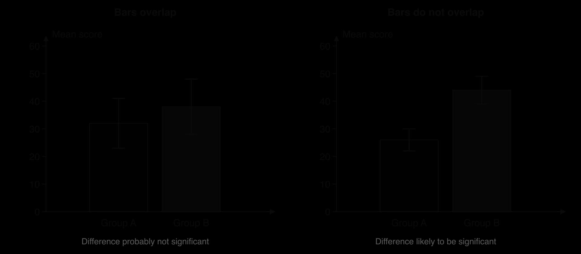
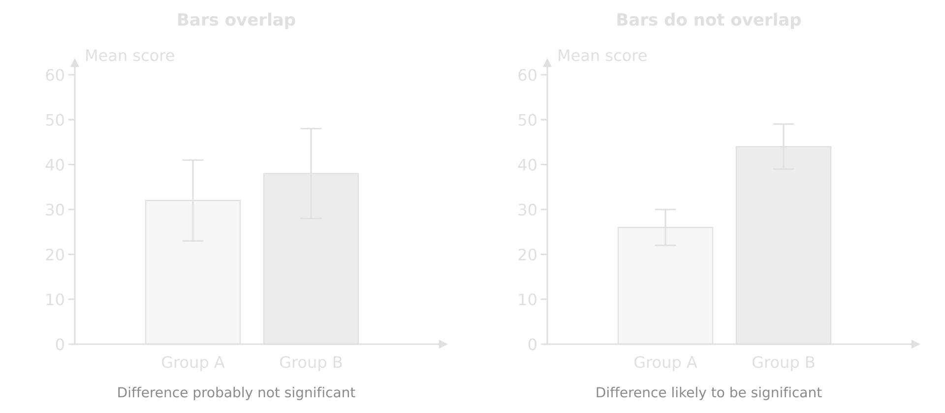
The rule of thumb is useful, but it has limits. It works best for independent groups. In a repeated-measures or cross-over design, the SD bars show how different the people are from each other, while the test compares each person with themselves. Two conditions can have overlapping SD bars and still differ significantly, if almost every participant changed in the same direction. Standard error (SE) bars are shorter than SD bars for the same data, because SE = SD ÷ √n, so check the caption before you judge overlap.

Statistical significance and p-values

The p-value is the probability of getting a difference at least as large as the one observed if the null hypothesis were true, that is, if there were really no effect. When p < 0.05, a result this large would happen by chance less than 5 times in 100, so the researchers reject the null hypothesis and call the result statistically significant. When p ≥ 0.05, the evidence is not strong enough to reject the null hypothesis.

Significance and size are different questions. With a large sample, a tiny difference can be significant but too small to matter to an athlete or a patient. With a small sample, a difference that would matter in a race can fail to reach significance. In an "evaluate" part, comment on both: is the effect significant, and is it big enough to be useful for health or performance?

Outliers

An outlier is a value that lies far from the rest of the data. In a 1B question you may be asked to point one out on a graph or in a table, suggest a cause (a measurement error, a participant who misunderstood the task, an injured or unusually trained participant) and say whether it should be kept. Remove an outlier only with a reason: if it came from an error in the method, removing it is justified; if it is a genuine but unusual result, it belongs in the data, and the conclusion should mention it.

Correlation is not causation

A correlation is a relationship between two variables in which they change together: a positive correlation when both rise together, a negative correlation when one rises as the other falls. The correlation coefficient r summarises the strength and direction, from −1 (perfect negative) through 0 (none) to +1 (perfect positive). A 1B question may give r with a critical value: if r (ignoring its sign) is greater than the critical value at p = 0.05, the correlation is significant.

Even a strong, significant correlation does not show causation. A third variable may cause both (a confounding variable), the direction of cause may be the reverse of what is assumed, or the link may be a coincidence. Sprinting ability, for example, could explain both fast approach speeds and long jumps in a group of long jumpers.

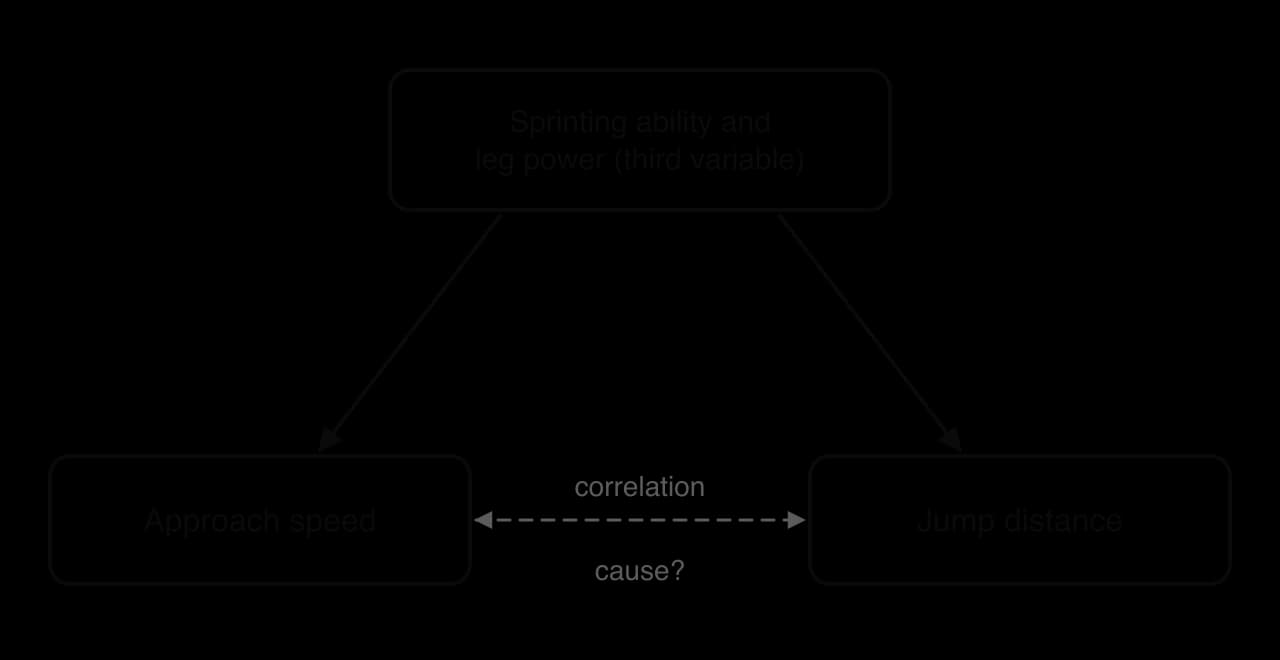
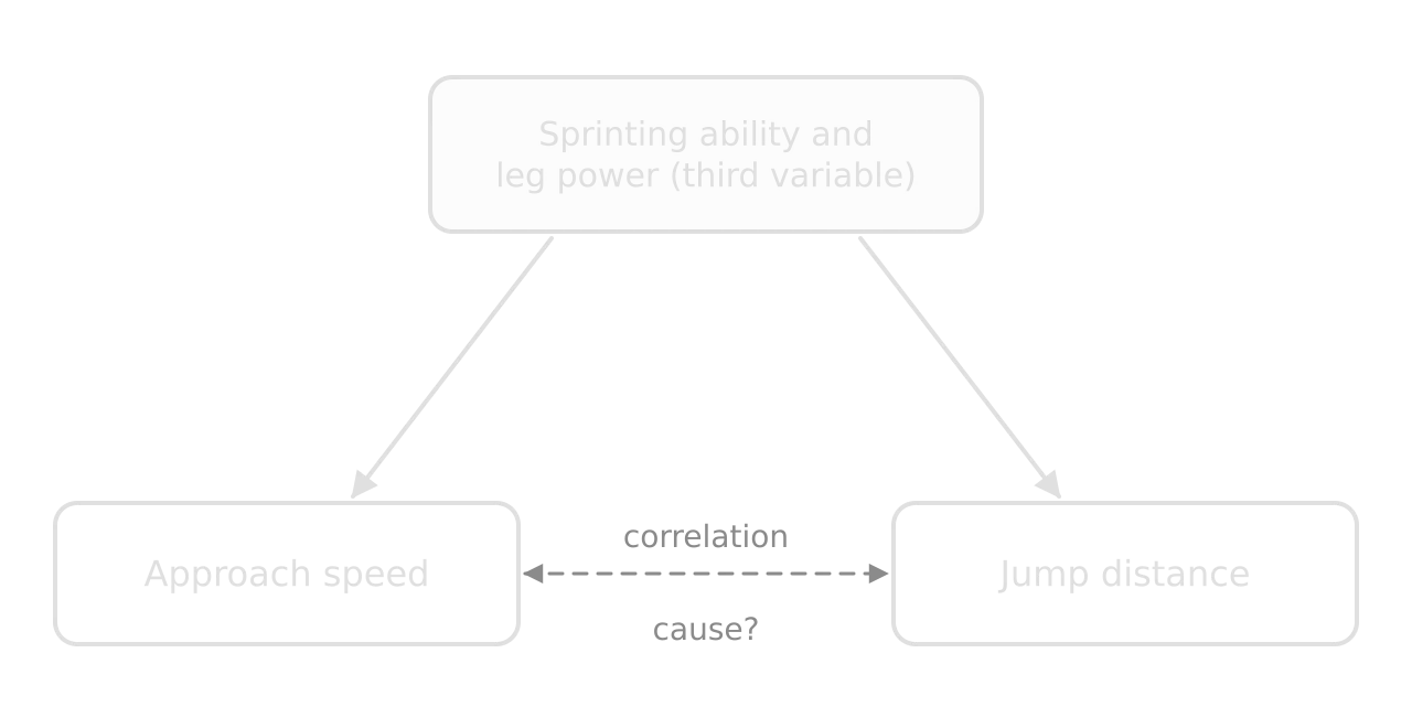
To show causation, researchers change one variable deliberately and keep the others constant, ideally with random allocation and a control condition. Correlational data are still valuable: they suggest which relationships are worth testing, and for some questions (the health effects of decades of activity, for example) an experiment would be impossible or unethical.

YouTube

Calculating from data

Calculation parts are the most reliable marks in Paper 1B, because the method is fixed. The marks are for the working, the answer and the unit. Write the equation or the method first, substitute the numbers with units, then give the answer to a sensible number of significant figures, usually the same as the least precise value in the data. Your calculator is allowed, and the data booklet gives the equations of motion, the coefficient of variation and the rules for uncertainties.

The calculations that appear most often are a mean, a difference, a percentage change, a ratio, a rate from a graph (a gradient), a speed or acceleration from the data booklet, and reading a value from a line of best fit. Percentage change always divides by the starting value:

A rate read from a graph is a gradient: the change in the y-value divided by the change in the x-value over the same interval, with the units of y per unit of x. On a heart rate–time graph, a rise of 25 beats min⁻¹ over 50 minutes is a rate of 0.5 beats min⁻¹ per minute. When the question says "estimate", a value read carefully from the graph within a small tolerance earns the mark; draw construction lines on the graph so the examiner can follow your reading.

Evaluating methods and suggesting improvements

The last parts of most 1B questions ask you to evaluate the method or the conclusion and to suggest an improvement. The language of evaluation is precise, and each word has its own meaning.

• Validity: whether the study measures what it claims to measure, and whether the conclusion follows from the design. A treadmill test in a cool laboratory may have low validity for predicting race performance in the heat.

• Reliability: whether repeating the measurement or the study gives similar results. A single trial per participant is less reliable than the mean of three.

• Accuracy: how close a measurement is to the true value. A badly calibrated scale gives inaccurate body mass.

• Precision: how close repeated measurements are to each other, and the smallest change the instrument can show (a stopwatch reading to 0.01 s, operated by hand).

Weaknesses come in two kinds. A random error varies unpredictably from one measurement to the next (reaction delay when hand-timing, day-to-day variation in sleep) and is reduced by repeating measurements and averaging. A systematic error shifts every measurement in the same direction (a heart rate monitor that reads 3 beats min⁻¹ high, a tape measured from the wrong mark) and is not reduced by repeats; it is reduced by calibration or a better method.

Improvements must be specific and realistic. "Use more participants" is weak on its own; "test at least 20 participants of each sex so the result can be applied to female athletes" is strong because it names the change and the reason. "Use better equipment" earns nothing; "replace hand timing with electronic timing gates to remove reaction-time error" earns the mark. Suggestions that would make the study impossible (testing every athlete in the country, measuring for ten years) are not realistic.

Sources: Costello, Bieuzen and Bleakley, European Journal of Sport Science, 2014.

A method for every 1B question

The same sequence works for any stimulus, from a sports nutrition trial to a study of goal setting.

1. Read the whole stimulus once. Mark the aim, the sample, the design, the independent and dependent variables, the controls and what the error bars show.

2. Read every part of the question before answering, and note the marks for each.

3. For describe and compare parts, quote values with units from the table or graph.

4. For calculations, write the method, substitute with units, and round sensibly.

5. For deduce parts, use the p-value or the critical value given, and say what it means for the null hypothesis.

6. For explain parts, link the result to the course mechanism or theory with "because… so…".

7. For evaluate and suggest parts, use the details of this method (its sample, controls, measures, setting), give the effect of each weakness, and finish with a judgment.

Practice set 1: fluid replacement and heart rate

The three practice sets are longer than a single question in the paper, so that each one covers every type of part. Each uses invented, hypothetical data. Try every part before opening the model answers, and time yourself: about 2 minutes per mark, the pace that fits an hour for the 25 marks of 1B.

The study

Researchers investigated the effect of drinking water during prolonged exercise on heart rate. Ten trained male cyclists (age 24 ± 3 years) completed two 60-minute rides on a cycle ergometer at a fixed power output that required 65% of their VO₂ max, in a laboratory kept at 30 °C and 50% relative humidity. The two trials were 7 days apart and started at the same time of day. The order of the trials was randomised.

• Fluid replacement (FR): the cyclists drank water every 10 minutes, in a volume equal to their sweat loss measured in a pilot ride.

• No fluid (NF): the cyclists drank nothing during the ride.

Heart rate was recorded with a chest-strap monitor every 10 minutes. Nude body mass was measured on scales (±0.1 kg) before and after each ride, after towelling dry. Rating of perceived exertion (RPE, Borg 6–20) and core temperature were recorded at 60 minutes. The results were compared with paired t-tests.

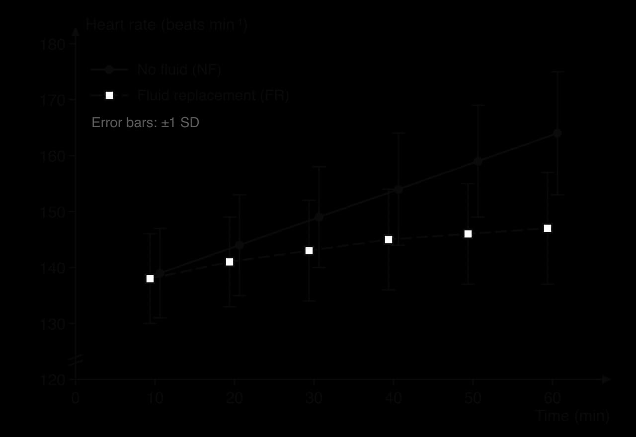
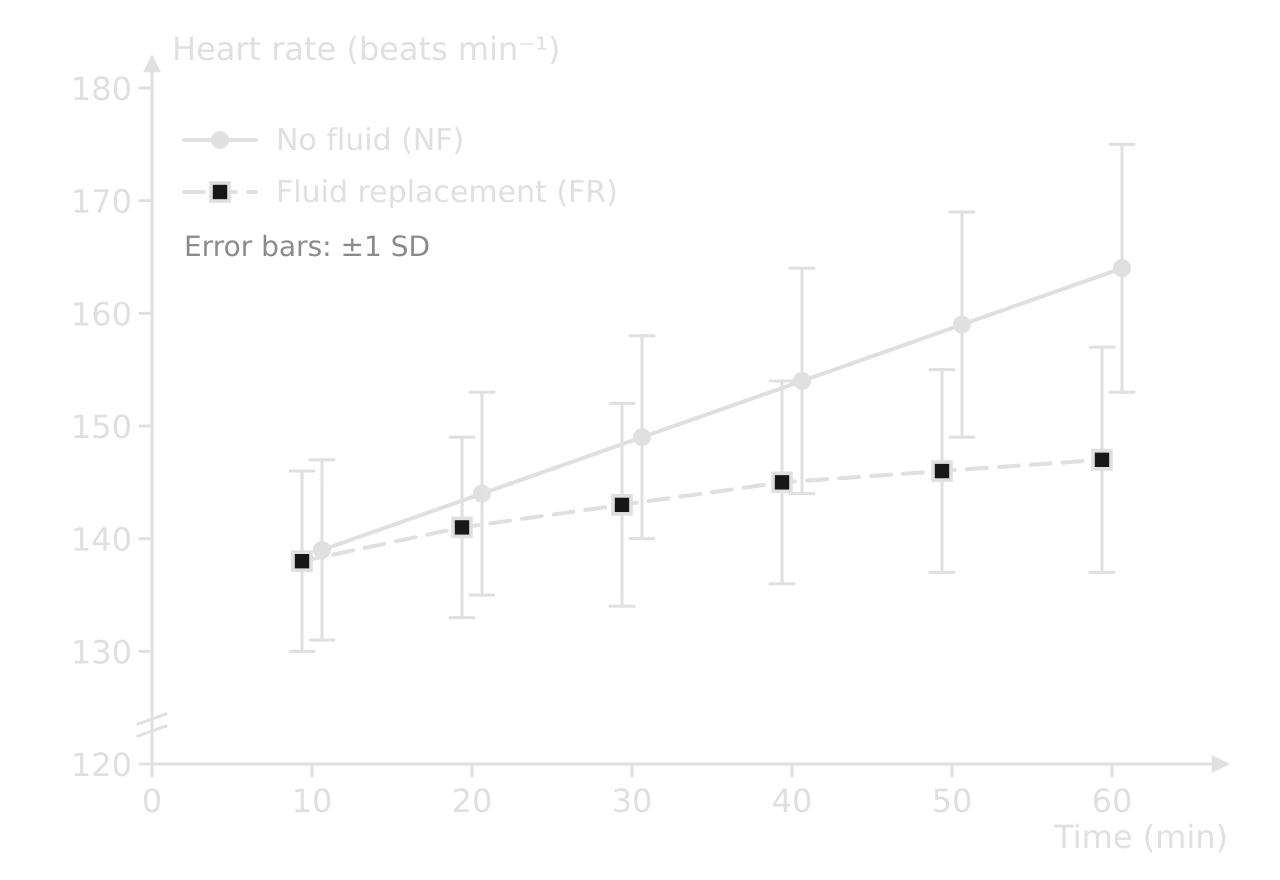
Table 1 gives the other results (hypothetical data, mean ± SD, n = 10).

Parts (e) to (h) ask about the statistics, the physiology behind the result and the quality of the design. Part (e) is the kind that separates strong candidates, because the error bars and the p-value appear to disagree.

Practice set 2: approach speed and long jump distance

The study

A biomechanist investigated the relationship between approach speed and jump distance in the long jump. Twelve club-level long jumpers (7 female, 5 male, age 17–23 years) each performed three competition-style jumps after their normal warm-up. Two timing gates were placed 6.00 m and 1.00 m before the take-off board, 5.00 m apart, at hip height. The time taken to pass between the gates was used to calculate the approach speed over the last 5 m. The distance of each jump was measured with a steel tape to the nearest 0.01 m. Each athlete's longest jump, with its approach speed, was used in the analysis.

Table 2 shows the timing gate data for three of the athletes (hypothetical data).

The scatter graph shows approach speed against jump distance for all twelve athletes. The Pearson correlation coefficient was r = 0.89. The critical value of r for 12 pairs of data (10 degrees of freedom) at p = 0.05 is 0.576.

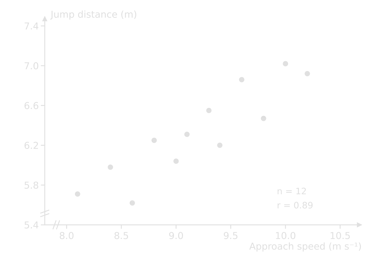
Parts (e) to (h) move from the data to the physics of projectiles and to the limits of what a correlation can show.

Practice set 3: blocked and random practice

The study

A motor learning researcher compared two practice schedules for learning three badminton serves: the low serve, the flick serve and the high serve. Twenty-four students aged 16–17 years with no badminton experience were randomly allocated to two groups of 12.

• Blocked group: practised all the trials of one serve, then all the trials of the next.

• Random group: practised the same number of trials of each serve, but in an unpredictable order.

Both groups completed six acquisition blocks of 18 serves (six of each type) over two days, with knowledge of results after every serve. Accuracy was measured as the radial error: the distance in centimetres from the centre of the target zone to where the shuttle landed, so a lower score is better. A retention test of 18 serves without feedback was held 48 hours after the last practice session.

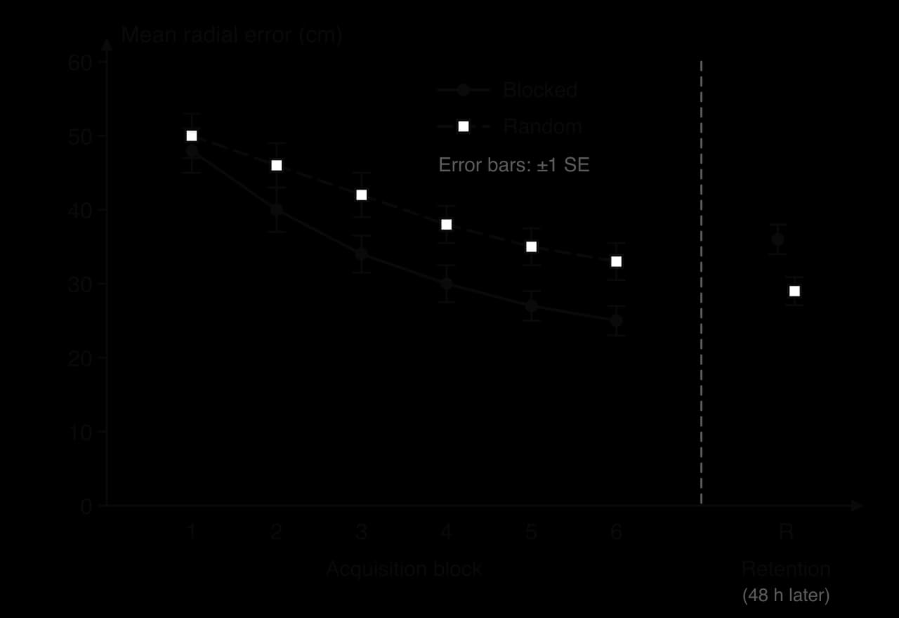
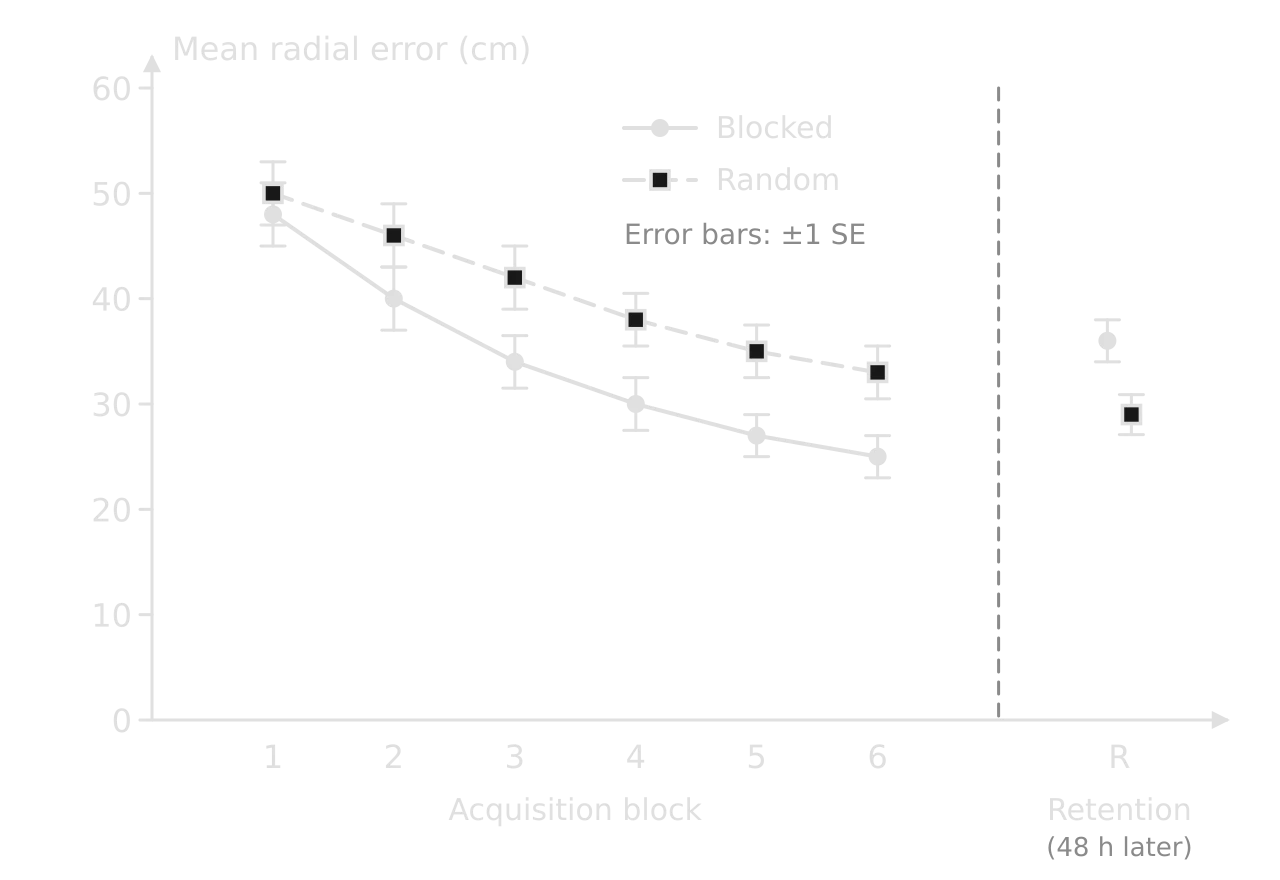
In the retention test, the mean radial error was 36 ± 7.0 cm in the blocked group and 29 ± 6.5 cm in the random group (mean ± SD). An independent t-test gave t = 2.54 with 22 degrees of freedom; the critical value of t at p = 0.05 is 2.074.

The final parts ask why the result occurred and how far it can be trusted. The explanation draws on the contextual interference effect and schema theory.

Checklist before you leave a 1B question

• To do:

  I can find the aim, sample, design, variables and controls in a study description.

• To do:

  I can describe a trend and compare two groups with values and units.

• To do:

  I can judge what overlapping or separated error bars suggest, and when the rule of thumb fails.

• To do:

  I can use a p-value or an r and its critical value to deduce whether a result is significant.

• To do:

  I can explain why a correlation does not show causation and name a likely third variable.

• To do:

  I can calculate a percentage change, a speed and a standard error with working and units.

• To do:

  I can evaluate a method with strengths, limitations linked to their effects, and a judgment.

• To do:

  I can suggest specific, realistic improvements and say why each would help.