Augment Education
    • Question bank
    • Quick fire
    • Worksheets
    • Flashcards
    • Notes
    • Try a quick-fire round
    • All features
    • Business
    • Digital Society
    • Economics
    • Geography
    • Global Politics
    • History
    • Philosophy
    • Psychology
    • Anthropology
    • World Religions
    • Biology
    • Chemistry
    • Physics
    • Computer Science
    • Design Technology
    • ESS
    • SEHS
    • Language and literature
    • Language acquisition
    • Maths AA
    • Maths AI
    • Dance
    • Film
    • Music
    • Theatre
    • Visual Arts
    • Grade calculator
    • Grade boundaries
    • Subject checker
    • Focus timer
    • Exam countdown
    • All free tools
    • IB guide
    • All subjects
  • Blog

Search

Search subjects, the syllabus, glossary terms, the booklets, the IB guide, help and the blog

Log inStart free
augment

Augment Education

IB Diploma revision built around the syllabus.

contact@augment-education.com

Product

  • Features
  • Question bank
  • Quick fire
  • Worksheets
  • Flashcards
  • Notes
  • Subjects
  • What's new

Learn

  • IB guide
  • Booklets, explained
  • Glossary
  • Blog
  • Free tools
  • Grade calculator
  • Subject checker

Company

  • About
  • Help
  • For parents
  • For teachers
  • Comparisons

Subjects

  • English A Lit
  • English A Lang & Lit
  • Chinese A Lit
  • Chinese A Lang & Lit
  • Spanish A Lit
  • Spanish A Lang & Lit
  • English Lit & Perf
  • Spanish Lit & Perf
  • English B
  • Mandarin B
  • Spanish B
  • English ab initio
  • Mandarin ab initio
  • Spanish ab initio
  • Business
  • Digital Society
  • Economics
  • Geography
  • Global Politics
  • History
  • Philosophy
  • Psychology
  • Anthropology
  • World Religions
  • Biology
  • Chemistry
  • Physics
  • Computer Science
  • Design Technology
  • ESS
  • SEHS
  • Maths AA
  • Maths AI
  • Dance
  • Film
  • Music
  • Theatre
  • Visual Arts

Augment Education is developed independently of the International Baccalaureate Organization and is not endorsed by it. “IB” and “International Baccalaureate” are its trademarks.

© 2026 Augment Education. All rights reserved.

  • Privacy
  • Terms
  1. Subjects
  2. SEHS
  3. Data analysis, statistics and the data booklet

Data analysis, statistics and the data booklet

Calculate and interpret averages, SD, coefficient of variation, SE, IQR, percentages and uncertainties, test significance with r and the t-test, draw and read graphs, and use the data booklet quickly in every paper.

  • IB Sports, Exercise and Health Science
  • Exam skills
  • SL and HL

36 min readLast reviewed 15 Oct 2026

Why numbers matter in SEHS

Every theme of the course rests on measurement: heart rate and VO₂ max in physiology, speed and force in biomechanics, questionnaire scores and accuracy in psychology and motor learning. These mathematical skills turn those measurements into evidence. They let you summarise a set of results, judge how variable and how certain they are, decide whether a difference or a relationship is real, and show it on a graph. They are examined in Paper 1B, can appear in any paper, and are the core of the data analysis in your scientific investigation.

Each skill is taught with a worked example using sport, exercise and health data (hypothetical unless a source is given) and the error students make most often. Your calculator handles the arithmetic; the marks are for choosing the right method, showing it and interpreting the answer.

Kinds of data and variables

Quantitative data are numbers (a time, a mass, a heart rate); qualitative data are descriptions (a participant reporting nausea, a coach's note that a jumper "stuttered" on the run-up). Quantitative variables are either continuous or discrete, and the difference decides how they are graphed and summarised.

Type

Meaning

SEHS examples

Usual graph

Continuous

Can take any value in a range; limited only by the precision of the instrument.

Sprint time (s), body mass (kg), VO₂ max (mL kg⁻¹ min⁻¹), core temperature (°C)

Scatter or line graph; histogram for a frequency distribution

Discrete

Can take only separate values, usually whole numbers or categories.

Number of successful free throws, push-ups completed, goals scored, Borg RPE (6–20)

Bar chart; values should not be joined by a line

Categorical (qualitative)

Groups with no numerical order, or an order without equal steps.

Sport played, sex, practice group, injury type

Bar chart or pie chart of counts or percentages

Common mistake

Joining the means of separate categories (football, rugby, hockey) with a line. A line implies that values between the points exist and follow a trend. Categories and discrete groups go on a bar chart; a line graph is for a continuous independent variable such as time, speed or work rate.

Units, symbols and numbers

SI units, prefixes and conversions

SEHS uses SI units: the metre, kilogram, second, newton, joule and watt, with prefixes from the data booklet (kilo- 10³, milli- 10⁻³, micro- 10⁻⁶ and so on). Units are written with a space and negative indices: m s⁻¹, m s⁻², mL kg⁻¹ min⁻¹, beats min⁻¹. The data booklet also gives the conversions you need most: 1 hour = 60 minutes = 3600 seconds, 1 litre = 1 dm³, 1 joule = 0.239 calories, and g = 9.81 m s⁻².

Worked example

Calculate (a) a runner's relative VO₂ max if her absolute VO₂ max is 3.6 L min⁻¹ and her body mass is 72 kg; (b) a speed of 36 km h⁻¹ in m s⁻¹; (c) a daily energy intake of 2,500 kJ in kilocalories (hypothetical values).

Show the solution

(a) Convert litres to millilitres, then divide by mass. 3.6 L min⁻¹ = 3,600 mL min⁻¹.

3,600 mL min−172 kg=50 mL kg−1 min−172 kg3,600 mL min−1​=50 mL kg−1min−1

(b) Convert kilometres to metres and hours to seconds. 36 km h⁻¹ = 36,000 m ÷ 3,600 s = 10 m s⁻¹. (Dividing a speed in km h⁻¹ by 3.6 gives m s⁻¹.)

(c) Use 1 J = 0.239 cal. 2,500 kJ × 0.239 = 598 kcal (597.5 kcal, rounded to 3 significant figures). This is a very low intake for an athlete, and in a nutrition question it would be worth commenting on.

Common mistake

Mixing minutes and seconds, or grams and kilograms, inside one calculation. A 400 m run in 1 min 05 s is 65 s, not 1.05 s. Convert every value to SI base units before substituting, and write the unit at every step so a mismatch is visible.

Scientific notation and orders of magnitude

Very large and very small numbers are written in scientific notation: a number between 1 and 10 multiplied by a power of 10. An adult has about 5 × 10⁹ red blood cells in each millilitre of blood and about 5 L (5 × 10³ mL) of blood, so the total is about (5 × 10⁹) × (5 × 10³) = 2.5 × 10¹³ red blood cells. Multiplying numbers in scientific notation means multiplying the first parts and adding the powers.

An order of magnitude is a factor of 10. Comparing to the nearest order of magnitude is a quick way to check whether an answer is sensible. A sarcomere is about 2.5 µm (about 10⁻⁶ m) long and a muscle fibre is roughly 10–100 µm (10⁻⁵ to 10⁻⁴ m) across, so a fibre is one to two orders of magnitude wider than a sarcomere is long. A resting cardiac output of 5 L min⁻¹ and an elite maximal output of 35 L min⁻¹ are of the same order of magnitude.

Significant figures and decimal places

Definition

Significant figures: the digits in a number that carry meaning about its precision, counted from the first non-zero digit; 0.0460 has three significant figures and 72.0 has three.

A calculated answer cannot be more precise than the data it came from. As a rule, give an answer to the same number of significant figures as the least precise value used. A distance of 5.00 m (3 significant figures) divided by a time of 0.49 s (2 significant figures) gives 10.204… m s⁻¹, which should be written 10 m s⁻¹ (2 significant figures), or 10.2 m s⁻¹ if the other values in the table are given to that precision. In a table of raw data, every value in a column is recorded to the same number of decimal places, matching the precision of the instrument.

Common mistake

Copying every digit from the calculator. "The mean jump height was 44.36363636 cm" claims a precision of a hundred-millionth of a centimetre from a tape that reads to the nearest centimetre. Write 44.4 cm (one more decimal place than the raw data is acceptable for a mean) or 44 cm.

Approximation, estimation and effects that can be ignored

Scientists often simplify a calculation by ignoring an effect that is small compared with the others. For a shot put, drag is tiny compared with the shot's weight, so the flight is treated as a projectile under gravity alone; for a badminton shuttle, drag is large and cannot be ignored. Estimating before calculating ("about 10 m s⁻¹ for a sprinter") catches slips such as a misplaced decimal point.

Fractions, ratios, percentages and reciprocals

Ratios compare two quantities: a work-to-rest ratio of 1:3 means 30 seconds of rest after a 10-second sprint. Percentages express a part of a whole out of 100: 18 successful serves out of 24 is 18 ÷ 24 × 100 = 75%. A reciprocal is 1 divided by a number, and it turns a quantity "per unit" into its inverse. Running pace and speed are reciprocals: a pace of 4.0 min km⁻¹ means 4.0 minutes for each kilometre, so the speed is 1 ÷ 4.0 = 0.25 km min⁻¹, which is 15 km h⁻¹ or 4.2 m s⁻¹.

Measures of central tendency

A measure of central tendency gives one typical value for a data set. The three in the course are the mean, the median and the mode.

Definition

Mean: the sum of all the values in a data set divided by the number of values; the most common measure of the typical value of a continuous variable.

  • The mean uses every value, so it is the most informative when the data are roughly symmetrical, but one extreme value can pull it a long way.

  • The median is the middle value when the data are in order (or the mean of the two middle values when there is an even number). It is not affected by extreme values, so it suits skewed data and data with outliers.

  • The mode is the most frequent value. It is the only average for categorical data (the most common injury type) and can be misleading for small sets of continuous data.

Worked example

The countermovement jump heights of 11 basketball players were (in cm, hypothetical data): 42, 38, 45, 51, 38, 47, 40, 44, 49, 38, 56. Calculate the mean, median, mode and range.

Show the solution

Step 1: put the data in order. 38, 38, 38, 40, 42, 44, 45, 47, 49, 51, 56.

Step 2: mean. Sum = 488 cm; 488 ÷ 11 = 44.36… = 44.4 cm.

Step 3: median. With 11 values the median is the 6th: 44 cm.

Step 4: mode. 38 cm appears three times: 38 cm.

Step 5: range. 56 cm − 38 cm = 18 cm.

The mode is far below the mean and median, so here it is a poor summary: three players happen to share the lowest score. The mean and median are close, which shows the data are roughly symmetrical, with the 56 cm player pulling the mean slightly above the median.

Measures of spread

Two teams can have the same mean jump height but very different players. Measures of spread (dispersion) describe how far the values are scattered. The course uses five: the range, the standard deviation, the coefficient of variation, the standard error and the interquartile range.

Range

The range is the largest value minus the smallest. It is quick to calculate but depends on only two values, so a single outlier changes it completely. It is used for error bars in some small data sets, and to describe the spread of repeated trials ("the three trials ranged from 41 to 46 kg").

Standard deviation

Definition

Standard deviation (SD): a measure of the spread of values around the mean of a data set; a small SD means the values are close to the mean, a large SD means they are widely spread.

For a sample of n values with mean xˉxˉ, the standard deviation s is:

s=∑(x−xˉ)2n−1s=n−1∑(x−xˉ)2​​

In words: find how far each value is from the mean, square those deviations so they are all positive, add them, divide by n − 1, and take the square root. Dividing by n − 1 instead of n corrects for the fact that a sample tends to underestimate the spread of the whole population. In practice you use a calculator (the sx or σn−1 key) or a spreadsheet (STDEV.S); the formula is not in the data booklet, but you must know what SD means and how to use it.

Worked example

A participant recorded five handgrip strength trials (kg, hypothetical data): 41, 44, 43, 46, 41. Calculate the mean and the standard deviation.

Show the solution

Step 1: mean. (41 + 44 + 43 + 46 + 41) ÷ 5 = 215 ÷ 5 = 43.0 kg.

Step 2: deviations and squared deviations.

x (kg)

x − x̄ (kg)

(x − x̄)² (kg²)

41

−2

4

44

1

1

43

0

0

46

3

9

41

−2

4

Sum

0

18

Step 3: divide by n − 1 and take the square root.

s=185−1=4.5=2.12 kgs=5−118​​=4.5​=2.12 kg

Answer: 43.0 ± 2.1 kg (mean ± SD). The deviations always add up to zero, which is a useful check on step 2.

Common mistake

Using the population key (σn or σx) on a calculator for a sample. For the grip data it gives 1.9 kg instead of 2.1 kg. Almost all data in SEHS are samples, so use sx (σn−1) or STDEV.S, and state which you used in an investigation.

When data follow a normal distribution, the SD gives a precise picture of where most values lie. The data booklet shows the normal distribution with its three bands.

−4−3−2−10123400.20.40.60.81SDs from the meanFrequency−1 SD+1 SD−2 SD+2 SD−3 SD+3 SD
  • Normal distribution
A normal distribution: about 68% of values lie within 1 SD of the mean, about 95% within 2 SD and about 99.7% within 3 SD. The narrower the curve, the smaller the SD.

If the VO₂ max of a large group of young adults is normally distributed with a mean of 45 mL kg⁻¹ min⁻¹ and an SD of 6 mL kg⁻¹ min⁻¹ (hypothetical values), about 68% of them lie between 39 and 51 mL kg⁻¹ min⁻¹ and about 95% between 33 and 57 mL kg⁻¹ min⁻¹. A person at 60 mL kg⁻¹ min⁻¹ is 2.5 SDs above the mean, which puts them among the top 1% or so of the group. Many fitness test norm tables are built this way.
YouTube
CrashCourse Statistics on range, interquartile range, variance and standard deviation, and why spread matters as much as the average.

Coefficient of variation

The SD is in the units of the data, so it cannot compare the spread of two different measures. An SD of 0.08 s in 20 m sprint times and an SD of 5.1 cm in jump heights cannot be compared directly. The coefficient of variation solves this by expressing the SD as a percentage of the mean. The data booklet gives it as:

V=100×SDmeanV=mean100×SD​

Definition

Coefficient of variation (V): the standard deviation expressed as a percentage of the mean, V=100×SDmeanV=mean100×SD​; it compares the relative spread of data sets with different units or different means.

Worked example

A squad's 20 m sprint times were 3.12 ± 0.08 s and their countermovement jumps 42 ± 5.1 cm (mean ± SD, hypothetical data). Determine which measure varied more within the squad.

Show the solution

Step 1: coefficient of variation for the sprint.

V=100×0.08 s3.12 s=2.6%V=3.12 s100×0.08 s​=2.6%

Step 2: coefficient of variation for the jump.

V=100×5.1 cm42 cm=12%V=42 cm100×5.1 cm​=12%

Step 3: compare. The units cancel, so the two percentages can be compared: the jump heights varied about four to five times more, relative to their mean, than the sprint times. A coach would expect players to differ more in jumping ability than in sprinting in this squad.

The coefficient of variation is also the usual way to report the reliability of a test. If an athlete repeats the same test several times, a low V between trials shows that the test gives consistent results. There is no single agreed cut-off for good reliability: the acceptable value depends on how small a change the test needs to detect, so a test meant to detect a 2% improvement needs a lower V between trials than one meant to detect a 10% improvement.

Common mistake

Comparing two SDs measured in different units or on very different means and concluding that the larger SD means more variation. An SD of 5.1 cm is not "bigger" than an SD of 0.08 s; they cannot be compared. Use the coefficient of variation.

Standard error

Definition

Standard error (SE): an estimate of how precisely a sample mean represents the population mean, calculated as the standard deviation divided by the square root of the sample size, SE=SDnSE=n​SD​.

The SD describes the spread of individual values. The standard error describes the uncertainty in the mean itself: if the study were repeated with a new sample, how much would the mean change? Because SE = SD ÷ √n, the standard error falls as the sample gets bigger, while the SD does not. A sample of 16 participants with an SD of 6.2 beats min⁻¹ has an SE of 6.2 ÷ √16 = 6.2 ÷ 4 = 1.55 beats min⁻¹. The formula is not in the data booklet.
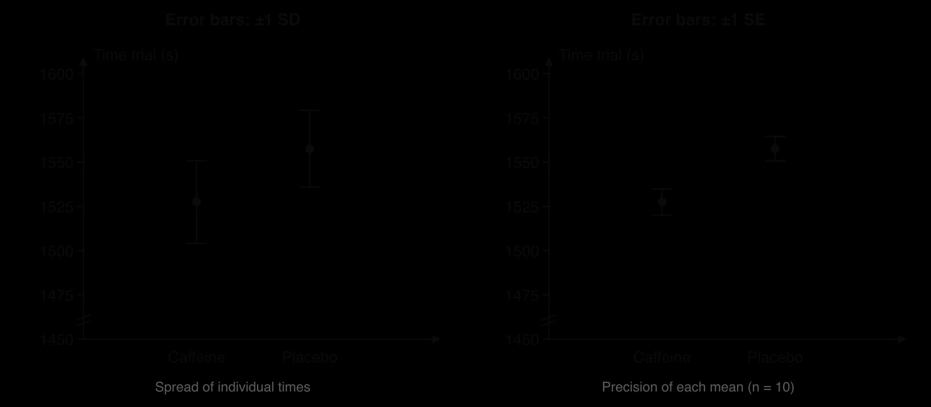
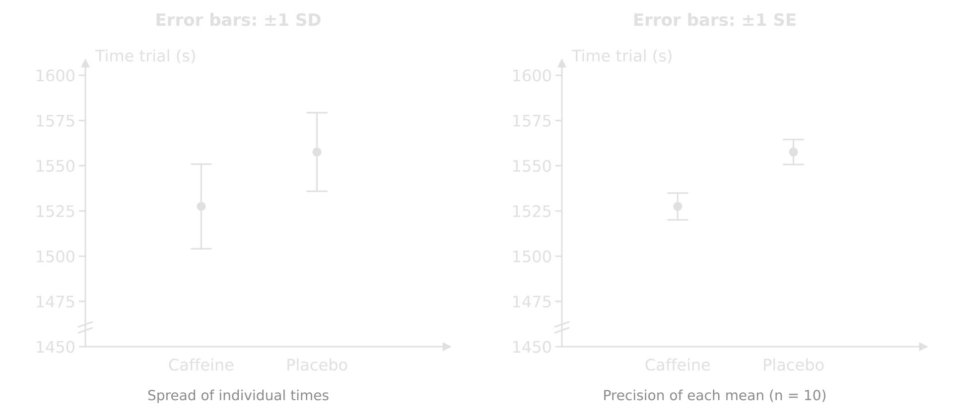
The same two hypothetical means, caffeine 1527.5 s and placebo 1557.6 s, plotted twice. Left with plus or minus 1 SD bars (about 22 to 23 s) that overlap. Right with plus or minus 1 SE bars (about 7 s) that do not overlap.The same two hypothetical means, caffeine 1527.5 s and placebo 1557.6 s, plotted twice. Left with plus or minus 1 SD bars (about 22 to 23 s) that overlap. Right with plus or minus 1 SE bars (about 7 s) that do not overlap.
The same hypothetical means plotted with SD bars and with SE bars. SE bars are shorter by a factor of √n (here √10). Always state which bars a graph shows.

The figure shows why the caption of a graph matters. With SD bars, the caffeine and placebo groups overlap, which shows that many individual cyclists in the two groups had similar times. With SE bars, the means are clearly separated, which suggests that the group means are precise enough to differ. Both versions are correct: SD bars show how different the people were, and SE bars show how certain the means are.

Interquartile range

Definition

Interquartile range (IQR): the difference between the upper quartile (Q3) and the lower quartile (Q1) of an ordered data set; it is the range of the middle 50% of the values and is not affected by extreme values.

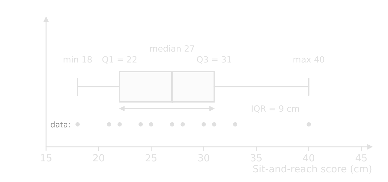
The quartiles divide ordered data into four equal parts, as the data booklet's diagram shows: Q1 has 25% of the values below it, the median (Q2) 50% and Q3 75%. The interquartile range is Q3 − Q1. It is the measure of spread that goes with the median, and it is shown on a box plot.
Worked example

Eleven students recorded these sit-and-reach scores (cm, hypothetical data): 25, 31, 18, 27, 40, 22, 30, 24, 33, 21, 28. Calculate the median and the interquartile range.

Show the solution

Step 1: order the data. 18, 21, 22, 24, 25, 27, 28, 30, 31, 33, 40.

Step 2: median. The 6th of 11 values: 27 cm.

Step 3: quartiles. Q1 is the median of the five values below the median (18, 21, 22, 24, 25): 22 cm. Q3 is the median of the five values above it (28, 30, 31, 33, 40): 31 cm.

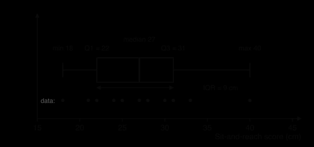
Step 4: IQR. 31 cm − 22 cm = 9 cm. The range is 40 − 18 = 22 cm; the IQR is much smaller because it ignores the extreme score of 40 cm.

Box plot of 11 hypothetical sit-and-reach scores on a scale from 15 to 45 cm: minimum 18, lower quartile 22, median 27, upper quartile 31, maximum 40, with the interquartile range of 9 cm marked under the box and the 11 data points shown as dots.Box plot of 11 hypothetical sit-and-reach scores on a scale from 15 to 45 cm: minimum 18, lower quartile 22, median 27, upper quartile 31, maximum 40, with the interquartile range of 9 cm marked under the box and the 11 data points shown as dots.
A box plot of the sit-and-reach data: the box spans Q1 to Q3 (the IQR), the line inside is the median and the whiskers reach the minimum and maximum. The long right whisker shows the single high score.

Tip

Pair the measures: mean with SD (or SE) for roughly symmetrical continuous data; median with IQR for skewed data or data with outliers; mode for categories.

Percentage change, difference and error

Percentages appear in almost every 1B question. Three different calculations share the word, and each divides by a different value.

Percentage change

Percentage change measures how much a value has risen or fallen relative to where it started, so it is the right calculation for any before-and-after comparison.

Definition

Percentage change: the change in a value expressed as a percentage of its original value, new−originaloriginal×100originalnew−original​×100; positive for an increase, negative for a decrease.

Worked example

After a 12-week walking programme, a participant's resting heart rate fell from 72 to 63 beats min⁻¹ (hypothetical data). Calculate the percentage change.

Show the solution
63−7272×100=−9 beats min−172 beats min−1×100=−12.5%7263−72​×100=72 beats min−1−9 beats min−1​×100=−12.5%

Answer: a decrease of 12.5% (or −12.5%). Dividing by the new value (63) gives −14.3%, the most common error.

Percentage difference

Percentage difference compares two values when neither is the "original", for example two methods of measuring the same thing, or two athletes. It divides the difference by the mean of the two values:

percentage difference=∣a−b∣(a+b2)×100percentage difference=(2a+b​)∣a−b∣​×100

Definition

Percentage difference: the absolute difference between two values divided by their mean and multiplied by 100; used to compare two values when neither is a reference or starting value.

If a 100 m run is timed at 11.42 s by hand and at 11.66 s by electronic timing (hypothetical values), the percentage difference is 0.24 ÷ 11.54 × 100 = 2.1%. Hand timing usually gives faster times, because the timekeeper reacts to the start signal late but anticipates the finish.

Percentage error

Definition

Percentage error: the difference between a measured value and the accepted or true value, expressed as a percentage of the accepted value; it shows how accurate a measurement is.

percentage error=∣measured value−accepted value∣accepted value×100percentage error=accepted value∣measured value−accepted value∣​×100

Worked example

A runner's GPS watch recorded 5.21 km for a certified 5.00 km course (hypothetical data). Calculate the percentage error of the watch.

Show the solution
∣5.21−5.00∣ km5.00 km×100=4.2%5.00 km∣5.21−5.00∣ km​×100=4.2%

Answer: 4.2%. The watch overestimates distance, so a runner trusting it would think their pace was about 4% faster than it was. A percentage error tells you about accuracy, not precision: the watch could give 5.21 km every time (precise) and still be wrong (inaccurate).

Common mistake

Using the three percentages interchangeably. Percentage change divides by the original value (before and after), percentage difference divides by the mean of two values (two methods, two people), and percentage error divides by the accepted value (a measurement against a known true value).

Uncertainty in measurements

Definition

Uncertainty: the range within which the true value of a measurement is expected to lie, written as ± after the value; the absolute uncertainty is in the units of the measurement, and the percentage uncertainty is the absolute uncertainty divided by the value, × 100.

No measurement is exact. Every value recorded in an investigation has an uncertainty, written as a range: 72.4 ± 0.1 kg. The uncertainty of a single reading depends on the instrument. For a digital instrument it is usually the smallest reading it can show (± 0.1 kg for scales that read to 0.1 kg). For an analogue scale such as a tape measure, it is usually half the smallest division (± 0.5 mm on a tape marked in millimetres), unless the method makes it larger. Human timing adds reaction time, so a hand-held stopwatch reading to 0.01 s is often given an uncertainty of about ± 0.2 s.

When a measurement is repeated, the spread of the repeats also gives an estimate of the uncertainty: half the range of the repeats is a common choice. Uncertainties are usually rounded to one significant figure, and the value is given to the same decimal place as its uncertainty: 6.6 ± 0.1 m s⁻¹, not 6.637 ± 0.1 m s⁻¹.

Percentage uncertainty compares the uncertainty with the size of the measurement. A hand-timed 12.4 ± 0.2 s has a percentage uncertainty of 0.2 ÷ 12.4 × 100 = 1.6%. The same ± 0.2 s on a 3.1 s sprint would be 6.5%, which is why hand timing is unsuitable for short sprints.

Propagating uncertainties

When measured values are combined in a calculation, their uncertainties combine too. The data booklet gives three rules:

If the calculation is…

then the uncertainty is…

In words

y=a±by=a±b
Δy=Δa+ΔbΔy=Δa+Δb

For a sum or difference, add the absolute uncertainties.

y=abcy=cab​
Δyy=Δaa+Δbb+ΔccyΔy​=aΔa​+bΔb​+cΔc​

For a product or quotient, add the fractional (or percentage) uncertainties.

y=any=an
Δyy=∣nΔaa∣yΔy​=​naΔa​​

For a power, multiply the fractional uncertainty by the power.

Worked example

Sum or difference. A cyclist's body mass is 72.4 ± 0.1 kg before a ride and 71.3 ± 0.1 kg after it. Calculate the mass lost, with its uncertainty.

Show the solution

Step 1: the value. 72.4 kg − 71.3 kg = 1.1 kg.

Step 2: the uncertainty. For a difference, add the absolute uncertainties: Δy = 0.1 kg + 0.1 kg = 0.2 kg.

Answer: 1.1 ± 0.2 kg. The uncertainty is about 18% of the mass lost, although each weighing was precise to 0.1%. Subtracting two similar numbers makes the relative uncertainty much larger.

The second rule applies to every equation in the data booklet that multiplies or divides, such as speed, acceleration, force, momentum and power. Fractional uncertainties are added because a small error in either the top or the bottom of a fraction changes the answer by a similar fraction.

Worked example

Quotient. An athlete runs 30.0 ± 0.1 m in 4.52 ± 0.05 s, measured with timing gates. Calculate the mean speed and its uncertainty.

Show the solution

Step 1: the value.

s=dt=30.0 m4.52 s=6.637 m s−1s=td​=4.52 s30.0 m​=6.637 m s−1

Step 2: add the fractional uncertainties.

Δss=0.130.0+0.054.52=0.0033+0.0111=0.0144sΔs​=30.00.1​+4.520.05​=0.0033+0.0111=0.0144

Step 3: convert to an absolute uncertainty. Δs = 0.0144 × 6.637 m s⁻¹ = 0.096 m s⁻¹, which rounds to 0.1 m s⁻¹.

Answer: 6.6 ± 0.1 m s⁻¹ (a percentage uncertainty of about 1.4%). Most of the uncertainty comes from the time, so improving the timing would improve the result most.

The third rule is needed when a measured value is squared or raised to another power. Body mass index (BMI) divides mass by height squared, so it combines the second and third rules.

Worked example

Power and quotient. A student has a mass of 68.0 ± 0.1 kg and a height of 1.75 ± 0.01 m. Calculate the BMI (mass ÷ height²) with its uncertainty.

Show the solution

Step 1: the value.

BMI=68.0 kg(1.75 m)2=22.2 kg m−2BMI=(1.75 m)268.0 kg​=22.2 kg m−2

Step 2: fractional uncertainty of height², using the power rule (n = 2).

Δ(h2)h2=∣2×0.011.75∣=0.0114h2Δ(h2)​=​2×1.750.01​​=0.0114

Step 3: add the fractional uncertainty of the mass.

ΔBMIBMI=0.168.0+0.0114=0.0015+0.0114=0.0129BMIΔBMI​=68.00.1​+0.0114=0.0015+0.0114=0.0129

Step 4: absolute uncertainty. 0.0129 × 22.2 = 0.29 kg m⁻², which rounds to 0.3 kg m⁻².

Answer: 22.2 ± 0.3 kg m⁻². The height measurement contributes almost all of the uncertainty, because it is squared and because ± 1 cm is a larger fraction of a height than ± 0.1 kg is of a mass.

Common mistake

Adding absolute uncertainties in a multiplication or division. For the speed example, adding 0.1 m and 0.05 s is meaningless, because the units differ. For any product or quotient, convert each uncertainty to a fraction (or percentage) of its value first, then add the fractions.

Exam tip

In Paper 1B you may be asked to state an uncertainty from an instrument, calculate a percentage uncertainty or propagate one through a data booklet equation. Write the rule you are using, show the fractional uncertainties, and round the final uncertainty to one significant figure with the value to the same decimal place.

Uncertainties and errors are linked but not the same. Random errors create uncertainty and show up as scatter between repeated readings, so repeating and averaging reduces their effect. Systematic errors shift every reading the same way and are invisible in the scatter: a heart rate monitor that reads 3 beats min⁻¹ high produces perfectly consistent but inaccurate data. Only calibration against a reference, or a better method, shows them up.

Proportionality and correlation

Direct and inverse proportionality

Two variables are directly proportional when doubling one doubles the other; the graph is a straight line through the origin. Newton's second law, F=maF=ma, gives an example: for a fixed mass, the force needed is directly proportional to the acceleration. Two variables are inversely proportional when doubling one halves the other. The time to cover a fixed distance is inversely proportional to speed, because t=dst=sd​.

012345678910111201020304050Speed (m s⁻¹)Time (s)4 m s⁻¹, 25 s8 m s⁻¹, 12.5 s
  • Time to run 100 m
Inverse proportion: doubling the speed from 4 to 8 m s⁻¹ halves the time for 100 m from 25 to 12.5 s. The curve never reaches either axis.

Many relationships in SEHS are neither: they rise and then level off (heart rate against time at a steady workload), or have a peak (performance against arousal). Proportional language should be kept for relationships that really are proportional.

Correlation and the correlation coefficient

Definition

Correlation: a relationship between two variables in which a change in one is associated with a change in the other; positive when both increase together, negative when one increases as the other decreases.

A scatter graph shows whether two continuous variables are correlated. The correlation coefficient r measures how closely the points follow a straight line, from +1 (a perfect positive line) to −1 (a perfect negative line); 0 means no linear relationship.
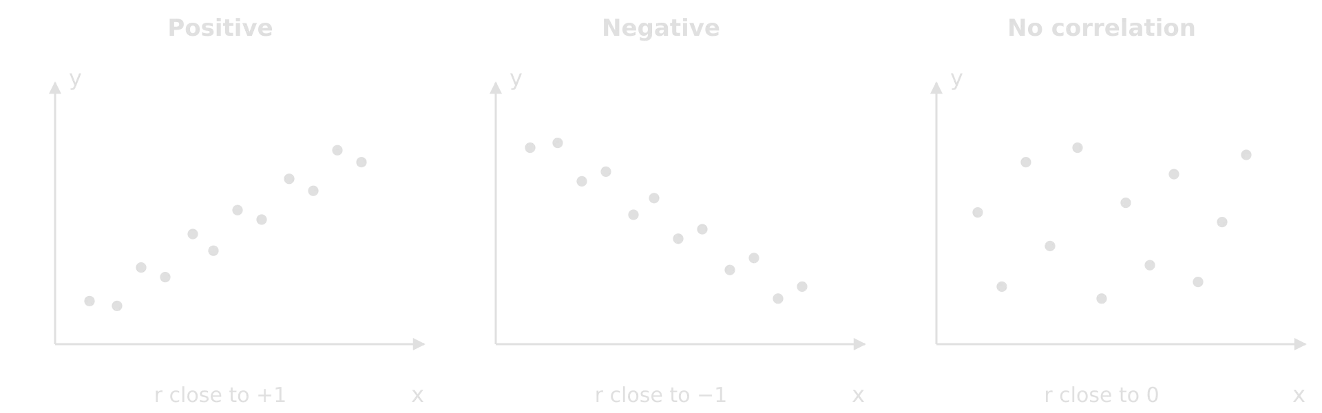
Three scatter graphs of y against x. Positive: points rise from bottom left to top right, r close to +1. Negative: points fall from top left to bottom right, r close to minus 1. No correlation: points scattered with no pattern, r close to 0.Three scatter graphs of y against x. Positive: points rise from bottom left to top right, r close to +1. Negative: points fall from top left to bottom right, r close to minus 1. No correlation: points scattered with no pattern, r close to 0.
Positive, negative and no correlation. The closer the points lie to a straight line, the closer r is to +1 or −1.

Definition

Correlation coefficient (r): a number from −1 to +1 that measures the strength and direction of the linear relationship between two variables; values near ±1 show a strong relationship and values near 0 a weak one.

A sample can show a correlation by chance, especially a small one, so r is compared with a critical value that depends on the number of pairs of data. The degrees of freedom are n − 2. If the size of r (ignoring its sign) is greater than the critical value at p = 0.05, the correlation is significant and the null hypothesis of no relationship is rejected. Critical values are given in the question when you need them; the table shows typical values for Pearson's r.

Pairs of data (n)

6

8

10

12

15

20

30

Degrees of freedom (n − 2)

4

6

8

10

13

18

28

Critical r at p = 0.05 (two-tailed)

0.811

0.707

0.632

0.576

0.514

0.444

0.361

Worked example

In a group of 8 recreational runners, weekly training distance and 10 km race time gave r = −0.68 (hypothetical data). Deduce whether the correlation is significant, and outline what it suggests.

Show the solution

Step 1: degrees of freedom. 8 − 2 = 6; the critical value at p = 0.05 is 0.707.

Step 2: compare. The size of r is 0.68, which is less than 0.707, so the correlation is not significant at p = 0.05; the null hypothesis cannot be rejected.

Step 3: interpret. The negative sign suggests that runners who trained further tended to run faster (lower times), but with only 8 runners the relationship could have arisen by chance. With 20 runners, the same r would be significant (critical value 0.444).

The coefficient of determination, R²

Definition

Coefficient of determination (R²): the proportion of the variation in the dependent variable that is explained by a trend line, from 0 to 1; for a straight line it equals r².

A spreadsheet adds R² to a trend line to show how well the line fits the data. R² = 0.80 means that 80% of the variation in the y-values is explained by the trend line, and 20% is due to other factors or random variation.

In a hypothetical study of 12 long jumpers with r = 0.89 between approach speed and jump distance, so R² = 0.89² = 0.79: about four-fifths of the differences in jump distance between the athletes go with differences in approach speed. Comparing R² for a straight line and a curve helps choose the better model, but a curve with more bends always fits slightly better, so the shape must also make physiological or physical sense.

Common mistake

Confusing r with R², or reading either as a percentage of cause. An R² of 0.79 does not mean that approach speed "causes 79% of jump distance". It means 79% of the variation is associated with the trend line. A correlation, however strong, does not show causation.

The t-test and statistical significance

A difference between two means could be a real effect of the independent variable or a chance result of which participants happened to be in the sample. A test of statistical significance decides between these. The test begins from the null hypothesis that there is no difference between the populations the samples came from.

Definition

t-test: a statistical test that compares two means and uses their difference, the spread of the data and the sample sizes to calculate t, which is compared with a critical value to decide whether the difference is significant.

The t-test produces a value of t: the larger t is, the less likely the difference is to be due to chance. The value of t is compared with a critical value for the degrees of freedom at p = 0.05. If t (ignoring its sign) is greater than the critical value, p < 0.05 and the difference is significant: the null hypothesis is rejected. A spreadsheet (for example the T.TEST function) gives the p-value directly.

Design

Which t-test

Degrees of freedom

Example

Two separate groups of people

Unpaired (independent) t-test

n₁ + n₂ − 2

A caffeine group and a placebo group

The same people measured twice

Paired t-test

n − 1 (number of pairs minus 1)

Flexibility before and after a training programme; a cross-over trial

For two groups of equal size, the unpaired t is the difference in means divided by its standard error:

t=xˉ1−xˉ2s12n1+s22n2t=n1​s12​​+n2​s22​​​xˉ1​−xˉ2​​

Worked example

Twenty trained cyclists were randomly allocated to take caffeine or a placebo (double-blind) before a 10 km time trial (hypothetical data). Caffeine: 1527.5 ± 23.4 s; placebo: 1557.6 ± 21.7 s (mean ± SD, n = 10 in each group). The critical value of t at p = 0.05 with 18 degrees of freedom is 2.101.

Calculate t and deduce whether caffeine had a significant effect.

Show the solution

Step 1: difference in means. 1557.6 s − 1527.5 s = 30.1 s.

Step 2: standard error of the difference.

23.4210+21.7210=54.8+47.1=10.1 s1023.42​+1021.72​​=54.8+47.1​=10.1 s

Step 3: t. 30.1 ÷ 10.1 = 2.98.

Step 4: compare. Degrees of freedom = 10 + 10 − 2 = 18. 2.98 > 2.101, so p < 0.05: the difference is significant and the null hypothesis is rejected. The caffeine group was 30.1 s, or 1.9%, faster. A cross-over design, with each cyclist doing both trials, would have been more powerful because it removes differences between cyclists.

A paired t-test uses the difference for each participant. t is the mean of the differences divided by its standard error, and the degrees of freedom are the number of pairs minus 1:

t=dˉ(sdn)t=(n​sd​​)dˉ​

Worked example

Eight participants completed a 6-week stretching programme. Their sit-and-reach scores (cm) before and after were (hypothetical data):

  • Before: 22, 18, 25, 30, 27, 20, 24, 28

  • After: 25, 21, 26, 34, 29, 24, 25, 31

Calculate t for a paired t-test and deduce whether the improvement is significant (critical t at p = 0.05 with 7 degrees of freedom = 2.365).

Show the solution

Step 1: differences (after − before). 3, 3, 1, 4, 2, 4, 1, 3 cm.

Step 2: mean and SD of the differences. Mean dˉdˉ = 21 ÷ 8 = 2.6 cm; SD sdsd​ = 1.19 cm (calculator, n − 1).

Step 3: t.

t=2.625(1.198)=2.6250.42=6.2t=(8​1.19​)2.625​=0.422.625​=6.2

Step 4: compare. 6.2 > 2.365, so the improvement is significant (p < 0.05). The means before and after (24.3 ± 4.1 and 26.9 ± 4.2 cm) have SDs larger than the change, yet the test is clearly significant, because every participant improved. Without a control group, though, the improvement could partly come from practising the test.

A significant result means the difference is unlikely to be due to chance in this sample. It does not mean the effect is large, important, or certain, and it does not show what caused it: that depends on the design (random allocation, controls, blinding). A non-significant result does not prove there is no effect; the sample may have been too small to detect it.

Exam tip

When a question gives a p-value or a t-value with its critical value, the deduce mark needs three things: the comparison ("p = 0.002 is less than 0.05" or "t = 2.98 is greater than 2.101"), the decision ("the difference is significant / the null hypothesis is rejected"), and what it means in context ("caffeine improved time-trial performance").

Graph skills

Choosing the right graph

Graph

Use it for

SEHS example

Bar chart

Comparing means or counts between categories or groups; add error bars to means.

Mean VO₂ max of rowers, runners and footballers

Histogram

The frequency distribution of one continuous variable; bars touch.

How many students scored in each 5 cm band of sit-and-reach

Scatter graph

The relationship between two continuous variables measured on the same individuals.

Approach speed and jump distance

Line graph

How a dependent variable changes with a continuous independent variable, often time.

Heart rate every minute during and after exercise

Pie chart

Proportions of a whole.

The percentage of injuries by body region in a season

Box plot

The median, quartiles and range of one or more data sets.

Reaction times of two age groups

Plotting a graph

A plotted graph needs the independent variable on the x-axis and the dependent variable on the y-axis, each with a label and a unit ("Heart rate (beats min⁻¹)"). Scales go up in equal steps that are easy to read (1, 2, 5 or 10 per square) and use most of the grid. An axis does not have to start at zero, but a break symbol shows when it does not. Points are plotted as small crosses or dots; if more than one data set shares the axes, each has its own symbol and a key, and the title says what the graph shows.

Sketch graphs

A sketch shows the general shape of a relationship on labelled axes without a scale: the inverted U, oxygen deficit and EPOC, heart rate before, during and after exercise, the path of a projectile. It still needs labelled axes with the variables (units are not needed without values), the correct shape, and the key features marked: a peak, a plateau, the point where exercise starts. Sketching is a drawing skill; plotting is a measuring skill.

Lines of best fit, gradients, intercepts and areas

A line of best fit shows the trend in scattered data. For a straight line, it passes through the middle of the points with about as many above as below; it does not have to pass through the origin or join the first and last points. A curve of best fit is drawn smoothly when the trend is clearly curved. The gradient of the line gives the rate of change of y with x, in the units of y divided by the units of x, and the intercept is the value of y where the line crosses the y-axis (when x = 0).

On a velocity–time graph the gradient is the acceleration and the area under the line is the displacement. The same ideas apply to other graphs: the gradient of a heart rate–time graph is the rate at which heart rate rises, and the area between an oxygen uptake curve and the steady-state demand is the oxygen deficit.
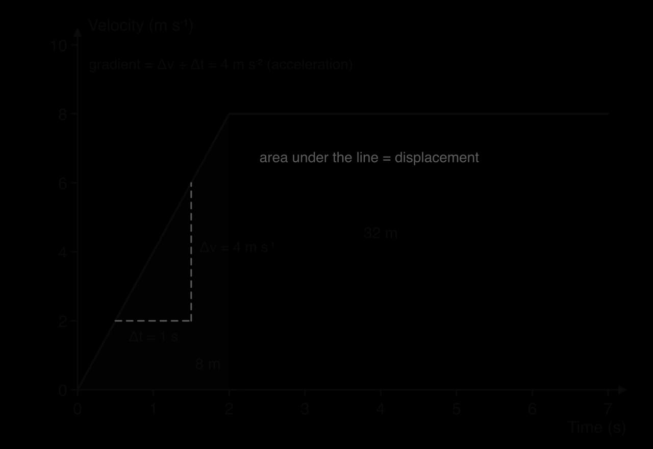
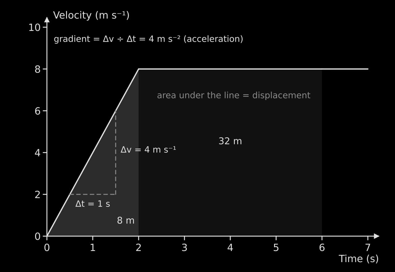
Velocity–time graph: velocity rises in a straight line from 0 to 8 m per s over 2 s, then stays at 8 m per s. A gradient triangle shows a rise of 4 m per s over 1 s, so 4 m per s squared. Shaded areas under the line are 8 m (triangle) and 32 m (2 to 6 s).Velocity–time graph: velocity rises in a straight line from 0 to 8 m per s over 2 s, then stays at 8 m per s. A gradient triangle shows a rise of 4 m per s over 1 s, so 4 m per s squared. Shaded areas under the line are 8 m (triangle) and 32 m (2 to 6 s).
A sprinter's idealised velocity–time graph. The gradient of the first part (Δv ÷ Δt) is the acceleration; the shaded areas under the line add up to the distance run, 8 m + 32 m = 40 m in 6 s.

Worked example

Using the velocity–time graph, calculate (a) the sprinter's acceleration in the first 2 s, and (b) the distance covered in the first 6 s.

Show the solution

(a) The velocity rises from 0 to 8 m s⁻¹ in 2 s. Using the data booklet:

a=(v−u)t=(8−0) m s−12 s=4 m s−2a=t(v−u)​=2 s(8−0) m s−1​=4 m s−2

(b) Area of the triangle (0–2 s) = ½ × 2 s × 8 m s⁻¹ = 8 m. Area of the rectangle (2–6 s) = 4 s × 8 m s⁻¹ = 32 m. Total = 40 m. The units of the area are (m s⁻¹) × s = m, which confirms it is a distance.

Plotting error bars

Error bars are drawn as a vertical line through each mean, from the mean minus the chosen measure to the mean plus it, with a short cap at each end. A mean of 147 beats min⁻¹ with an SD of 10 beats min⁻¹ has a bar from 137 to 157. The key or caption must say whether the bars show ±1 SD, ±1 SE, the range or the uncertainty of the instrument. On a scatter graph, horizontal and vertical bars can show the uncertainty in both variables; a line of best fit that passes through every bar is consistent with the data.

Interpolation and extrapolation

Interpolation reads a value from the line of best fit within the range of the data; it is usually reliable. Extrapolation extends the line beyond the data to predict a value; it assumes the trend continues, which may not be true. Submaximal fitness tests depend on extrapolation: heart rate is measured at several low work rates and the line is extended to the age-predicted maximum heart rate to estimate the maximal work rate or VO₂ max.
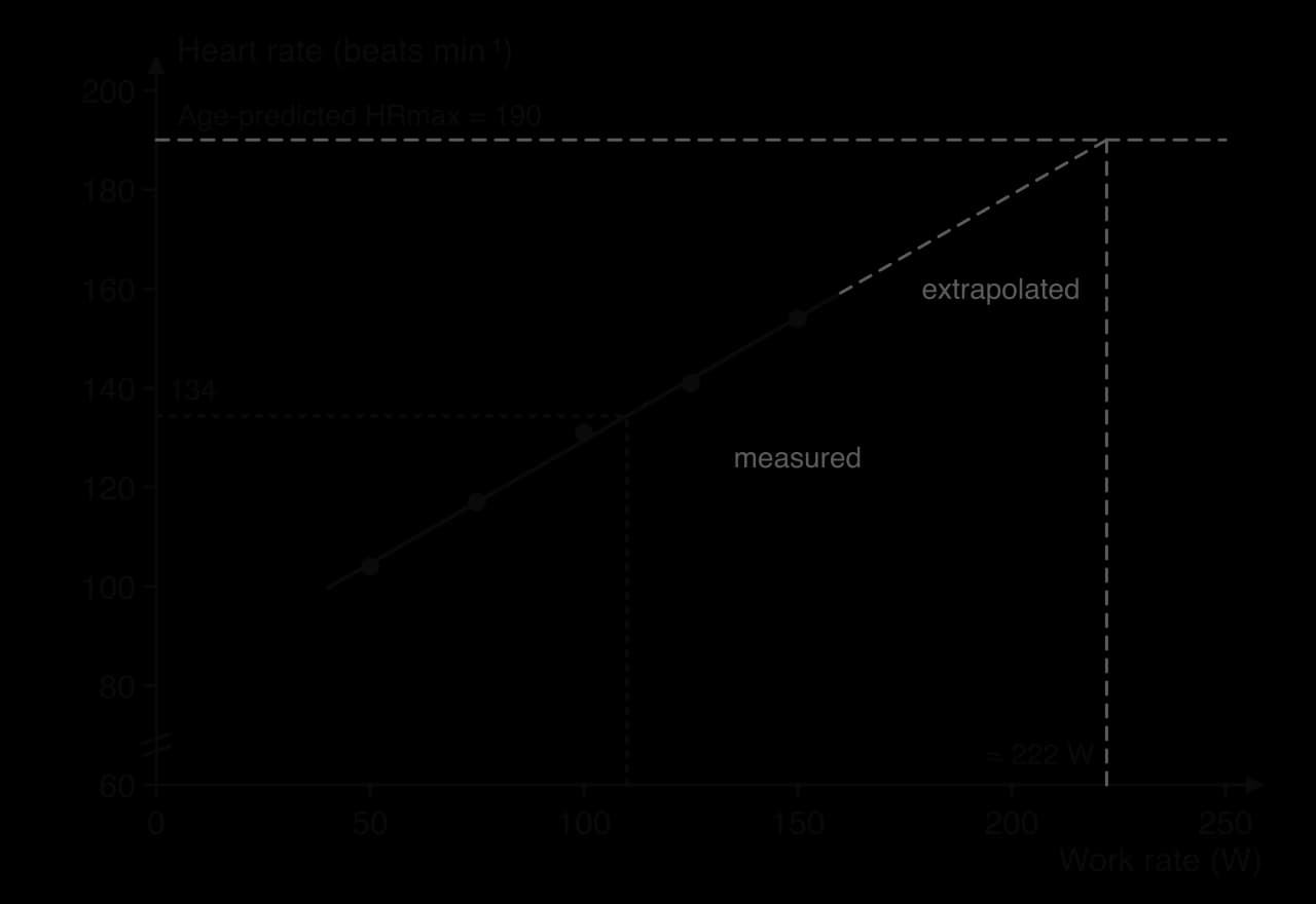
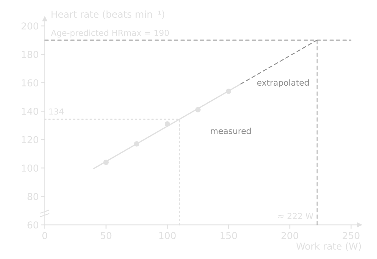
Hypothetical heart rate against work rate: five points from 104 at 50 W to 154 at 150 W with a straight best-fit line. Dotted lines read 134 beats per min at 110 W. A dashed extension meets a dashed line at age-predicted maximum 190 at about 222 W.Hypothetical heart rate against work rate: five points from 104 at 50 W to 154 at 150 W with a straight best-fit line. Dotted lines read 134 beats per min at 110 W. A dashed extension meets a dashed line at age-predicted maximum 190 at about 222 W.
Hypothetical submaximal cycle test. Interpolation at 110 W gives about 134 beats min⁻¹; extrapolating the line to an age-predicted maximum of 190 beats min⁻¹ estimates a maximal work rate of about 222 W.

Worked example

In the submaximal test shown, the line of best fit is HR = 0.50 × (work rate) + 80 (hypothetical data). (a) Estimate the heart rate at 110 W. (b) Determine the work rate at which the line reaches 190 beats min⁻¹. (c) Suggest why the estimate in (b) may be inaccurate.

Show the solution

(a) Interpolation. HR = 0.50 × 110 + 80 = 135 beats min⁻¹ (the more precise line, 0.496 × 110 + 79.8, gives 134; reading the graph gives about 134).

(b) Extrapolation. 190 = 0.50 × W + 80, so W = 110 ÷ 0.50 = 220 W (about 222 W from the precise line).

(c) The estimate assumes the heart rate–work rate line stays straight up to maximum, which may not hold near maximal effort, and it uses an age-predicted maximum heart rate (220 − age) that can differ from a person's true maximum by 10 beats min⁻¹ or more. Both errors are carried into the extrapolated value.

Common mistake

Treating an extrapolated value as a measurement. Any value read from beyond the plotted data is a prediction, and its uncertainty grows the further the line is extended. Say so in an answer, and give a reason why the trend might change (a plateau, a physiological maximum, a change in technique).

Graphs also have features worth naming in a description: a maximum or minimum (peak heart rate, the lowest blood glucose), a change in gradient (the point where blood lactate starts to rise sharply as intensity increases), a plateau (steady state) and an intercept (the resting value at time zero).

The data booklet

Every candidate has a clean copy of the SEHS data booklet in every paper. It is a reference, so it saves you memorising some content, but only if you know what is in it and where. The table lists its seventeen sections.

Section

Contents

Typical use in a question

1–5

Endocrine glands; structure of the heart (with the conduction system); cardiovascular system; respiratory system; digestive system

Label a structure, or trace a pathway such as the impulse from the SA node

6

Menstrual cycle: hormone levels across a 28-day cycle

Interpret hormone changes in a question on training or performance

7–9

Skeletal system (with vertebral regions); anatomical planes and axes; muscular system

Name the bones and muscles in a movement; state the plane and axis

10–11

Muscle fibre; sarcomere in a relaxed myofibril

Label the sarcomere; describe changes during contraction

12

Classes of lever

Classify a lever in a movement

13–14

SI multipliers; unit conversions and constants (1 h = 3600 s, 1 L = 1 dm³, 1 J = 0.239 cal, g = 9.81 m s⁻²)

Convert units; use g in Fg=mgFg​=mg

15

Equations of motion and mechanics; energy, work and power

Calculate speed, acceleration, force, momentum, impulse and, at HL, restitution, friction, work and power

16

Uncertainties: the three propagation rules

Combine uncertainties in a calculation

17

Variation in data sets: quartiles and IQR, the normal distribution (68/95/99.7%), the coefficient of variation

Interpret spread; calculate V

Some tools you need are not in the booklet: the formulas for the mean, standard deviation, standard error, percentage change, percentage difference and percentage error; how to carry out a t-test; and the critical value tables for t and r, which are given in the question when they are needed. These must be learned.

Exam tip

Use the data booklet actively. When a question asks you to calculate, find the equation in section 15 first and copy it into your answer with its symbols (p=mvp=mv, J=FΔtJ=FΔt). When a question asks you to label the heart, a lever or a sarcomere, check the booklet's diagram for the exact names. Before the exam, practise with your own copy until you can find any equation in a few seconds.

Tip

Annotate a practice copy of the data booklet (never the one in the exam room) with when to use each equation and one example each: "impulse: a sprinter in the blocks"; "coefficient of variation: comparing sprint and jump spread". Writing the uses yourself makes the equations easier to find under time pressure.

Add to your notes: a one-page table of every calculation in SEHS data analysis, with three columns: the formula (marking those given in the data booklet), when to use it, and the error to avoid. Include the mean, SD, V, SE, IQR, the three percentages, the three uncertainty rules, r against a critical value, R², and both t-tests.

Checklist: data analysis skills

  • To do:

    I can calculate a mean, median, mode and range, and choose the right average for the data.

  • To do:

    I can calculate and interpret a standard deviation, and use the 68–95–99.7% rule.

  • To do:

    I can calculate the coefficient of variation with the data booklet equation and use it to compare spread.

  • To do:

    I can calculate a standard error and explain how SE bars differ from SD bars.

  • To do:

    I can find the quartiles and interquartile range and draw a box plot.

  • To do:

    I can calculate percentage change, difference and error, and say which one a question needs.

  • To do:

    I can record uncertainties and propagate them with the data booklet rules.

  • To do:

    I can compare r with a critical value, interpret R² and explain why correlation is not causation.

  • To do:

    I can choose a paired or unpaired t-test, calculate t and interpret it at p = 0.05.

  • To do:

    I can plot and sketch graphs, draw lines of best fit, find gradients and areas, and interpolate and extrapolate with care.

Keep your place

In Augment the notes remember where you stopped and which pages you have finished.

Open in Augment

More IB SEHS notes

  • Paper 2: short-answer and extended-response questionsThe page before this.
  • Planning the scientific investigationThe next page.
  • SEHS assessmentEach SEHS paper, the internal assessment and grade boundaries.
  • IB SEHSThe SEHS syllabus, how it is assessed and every notes page.

Carry on with SEHS in Augment

With a free account, Augment remembers where you stopped in the notes and which questions you have marked.

Start free