Data analysis

The Data analysis criterion assesses how the raw data are recorded, how they are processed into the quantities that answer the research question, and how uncertainties are handled throughout. A top-band analysis is clear (a reader can follow every step) and precise (every number has a unit, a sensible number of significant figures and an uncertainty), and the processing is correct and relevant to the question.

Analysis turns a table of readings into evidence. The usual route is raw data, then means and uncertainties, then a graph that tests the predicted relationship, then a gradient or intercept with its uncertainty, and finally a derived quantity that can be compared with theory or an accepted value. Each step is shown once, with an explanation, so that a moderator can check it.

What the criterion rewards

"Clear" refers to how easily the reader follows the work: labelled tables, a sample of each calculation, graphs that are easy to read. "Precise" refers to the numbers themselves: units, decimal places consistent with the instruments, significant figures matched to the uncertainty. A beautifully presented analysis with numbers to eight significant figures is clear but not precise.

Recording raw data

Raw data go into a table as they are taken. A raw data table follows a few conventions that make it both clear and precise.

• Each column heading gives the quantity, its unit and its uncertainty: "$L$ / m ± 0.002". The unit appears only in the heading, not after each number.

• The independent variable is in the first column.

• Every value in a column has the same number of decimal places, set by the resolution of the instrument. A balance reading to 0.01 g gives 12.30 g, not 12.3 g.

• Repeated readings sit in adjacent columns ("Trial 1", "Trial 2", "Trial 3").

• Qualitative observations are recorded too: "the ball skidded at 14°", "the reading drifted by 0.02 Ω while the clip was held".

Qualitative data

Not all useful data are numbers. Observations such as "the trolley wobbled on the track above 0.8 m s⁻¹", "condensation formed on the beaker below 10 °C" or "the oscillation died away after about 15 cycles" explain anomalies, set the limits of a range and give the evaluation specific evidence. They are recorded with the quantitative data, at the time they are seen, and referred to where they matter in the analysis.

The uncertainty of a single reading

Every reading has an absolute uncertainty, written with ±, that reflects how precisely it can be read. For a digital instrument the usual convention is ± one unit in the last digit displayed. For an analogue scale it is commonly taken as ± half the smallest division, although a larger value is justified when the reading is harder to judge (a moving needle, a meniscus, two ends of an object both read on a rule).

The uncertainty from repeated readings

When repeated readings differ, the spread is a direct measure of the random uncertainty. A simple and widely accepted estimate is half the range:

The mean is the best estimate of the value, and it is quoted to the same decimal place as its uncertainty. For three readings of 1.85 Ω, 1.93 Ω and 1.98 Ω, the mean is 1.92 Ω and half the range is 0.065 Ω, so the result is $1.92\pm 0.07\mathrm{\Omega }$. If half the range is smaller than the uncertainty of a single reading, the reading uncertainty is used instead.

Outliers

An outlier is a reading that lies far from the trend of the others. An outlier is never deleted silently. It is identified, a reason is looked for (a misread scale, a slipped clamp, a different setting), and the reading is repeated if possible. If it is excluded from the processing, the report says so and gives the justification; if no reason can be found, it is usually kept and its effect discussed. No statistical test is expected for this, but the decision must be explained.

Processing data

Processing turns raw readings into the quantities that answer the question. It includes means, derived quantities (speed from distance and time, resistance from pd and current, $T^2$ or $1\mathrm{/}{d}^2$ for a linearised graph), and the uncertainty of each.

Propagating uncertainties

When a quantity is calculated from measured values, its uncertainty is found from theirs. The rules use absolute uncertainties ($\mathrm{\Delta }x$) for sums and differences, and fractional uncertainties ($\mathrm{\Delta }x\mathrm{/}x$) for products, quotients and powers.

Fractional uncertainties are often written as percentage uncertainties: a fractional uncertainty of 0.026 is a percentage uncertainty of 2.6%. Adding percentages is quick and makes it easy to see which measurement contributes most.

Squared and cubed quantities appear often in physics investigations, so identifying the measurement that is raised to a power is usually the first step in finding the largest source of uncertainty.

Showing the processing

The report shows one sample calculation of each type, with the numbers substituted and the units, followed by a table of all the processed values. Repeating the same calculation eight times uses space and words without adding anything.

Graphs

A graph is the main tool for testing a relationship. It shows the trend, the scatter and any outliers at a glance, and its gradient and intercept carry the quantitative result.

Drawing a good graph

• The independent variable goes on the horizontal axis and the dependent variable (or the processed quantity) on the vertical axis.

• Axes are labelled with the quantity and unit in the form "quantity / unit": "$R$ / Ω", "$1\mathrm{/}{d}^2$ / m⁻²".

• Scales are chosen so that the data fill most of the graph, with sensible steps (1, 2, 5 or 10 units per division). The origin is included when the theory says the line should pass through it.

• Error bars show the uncertainty of each point in each direction. If the bars in one direction are too small to draw, the report says so.

• A line of best fit (or a smooth curve of best fit) is drawn through the trend, with points scattered evenly on both sides. Points are never joined dot to dot.

• Several data sets on one graph are distinguished by different symbols and a key.

Graphs drawn with software are normal in a report. The software's trend line is acceptable as the best-fit line, but its equation must be interpreted, not just displayed: the gradient and intercept are quoted with units and with their uncertainties.

Using a spreadsheet

A spreadsheet makes processing fast and consistent: one formula, entered once and filled down a column, calculates every mean, every uncertainty and every transformed value in the same way. The report states which software was used and gives one sample calculation by hand, so that a reader can check the formula. Common functions include the mean (AVERAGE), the maximum and minimum of repeats (MAX, MIN) for half the range, and LN or POWER for transformed axes.

Spreadsheets can also add error bars from a column of uncertainties and draw a trend line. The maximum and minimum gradient lines are found by plotting two extra straight lines by eye, adjusting their gradients and intercepts until each one just passes through every error bar, and reading off the gradients. Some spreadsheets report a statistical uncertainty in the gradient (for example from LINEST); this can be quoted as well, if the report explains what it is, but it does not use the error bars and can differ from the maximum–minimum estimate.

Gradient and intercept with uncertainty

The gradient of the best-fit line is usually the key result. Its uncertainty comes from the error bars. Two further lines, the maximum and minimum gradient lines, are drawn through all the error bars: the steepest possible and the shallowest possible. The uncertainty in the gradient is then

The same lines give the uncertainty in the intercept, $\mathrm{\Delta }c=(c_{\text{max}}-c_{\text{min}})\mathrm{/}2$, taking the intercepts of the two lines. Some analyses use the difference between the best gradient and the maximum or minimum gradient instead; either method is acceptable if it is stated.

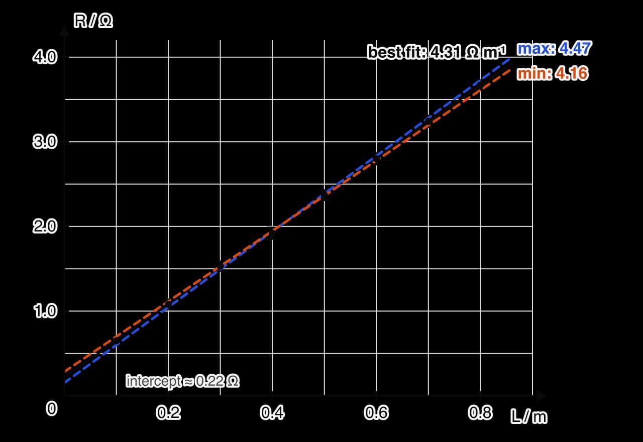
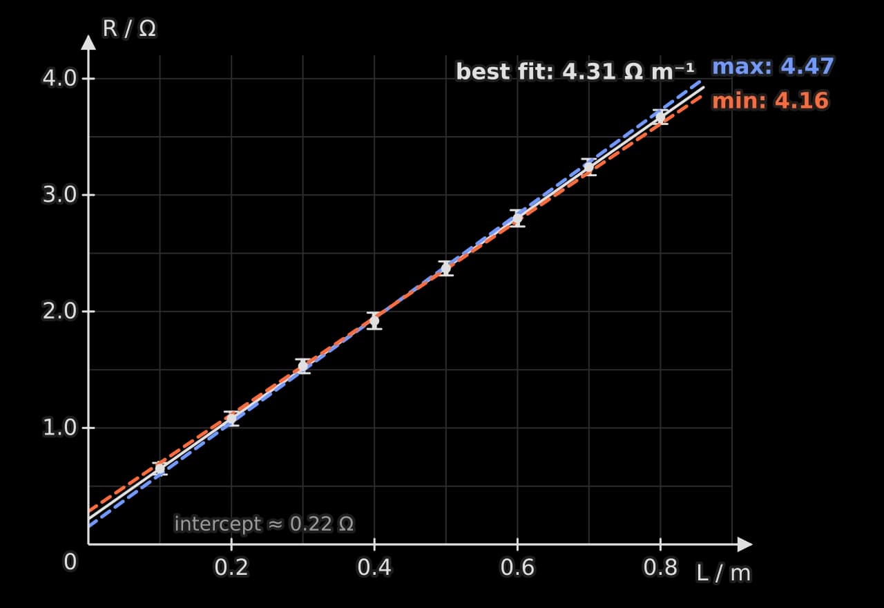
The resistance graph shows the method on sample data. The error bars in length (±0.002 m) are too small to see at this scale, so the maximum and minimum lines are set by the resistance error bars. The best-fit gradient is 4.31 Ω m⁻¹, and the steepest and shallowest lines that still pass through every error bar have gradients of 4.47 Ω m⁻¹ and 4.16 Ω m⁻¹, so

Interpreting a graph

The features of a graph each have a physical meaning, which the analysis states.

An intercept that does not match the theory is evidence of a systematic error. If the intercept, with its uncertainty, does not include zero when theory predicts zero, the report says so and suggests a cause. In the resistance data the intercepts of the two lines are 0.15 Ω and 0.28 Ω, so the intercept is $0.22\pm 0.07\mathrm{\Omega }$, clearly not zero, which matches the resistance of the leads and clip contacts.

Linearising a relationship

Many relationships in physics are not straight lines, but they can be rearranged into the form $y=mx+c$ by choosing what to plot. A straight line is much easier to judge by eye than a curve, it gives a gradient and intercept with uncertainties, and it tests the predicted relationship directly. Linearising is used only where theory predicts a form to test.

The light-intensity data show linearisation in action. Plotted directly, intensity against distance falls along a curve.

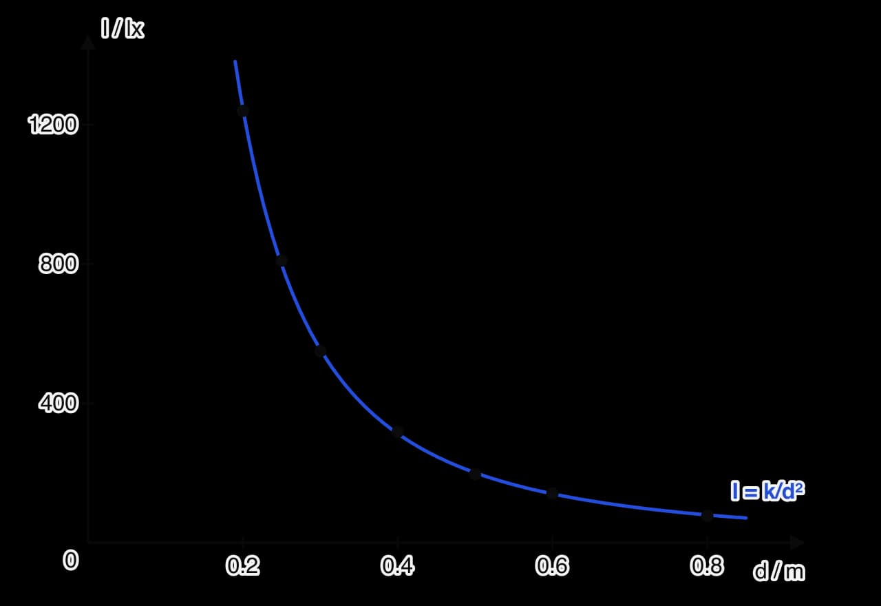
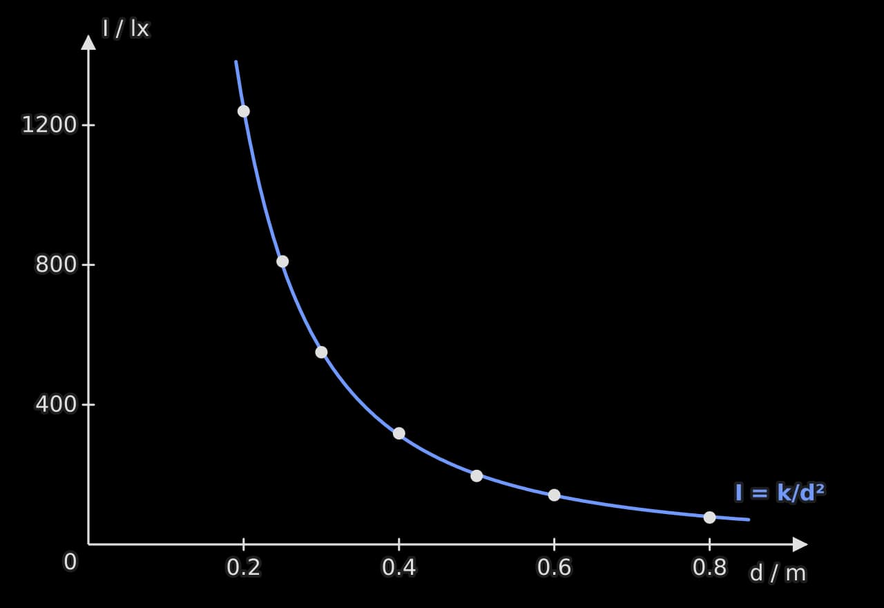
The curve has the expected shape, but a curve that falls steeply and levels off fits several models. If the lamp behaves as a point source, $I=k\mathrm{/}{d}^2$, so plotting $I$ against $1\mathrm{/}{d}^2$ should give a straight line through the origin.

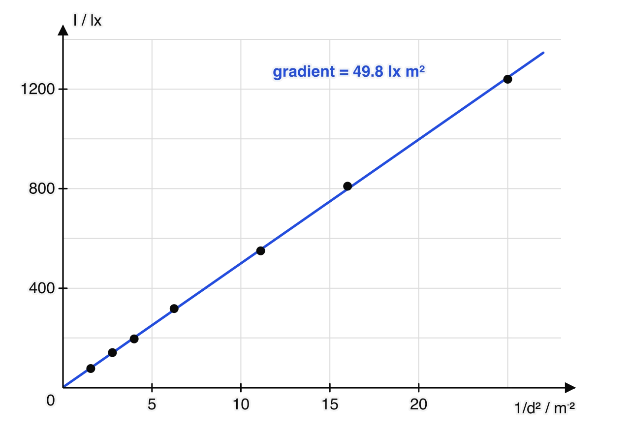
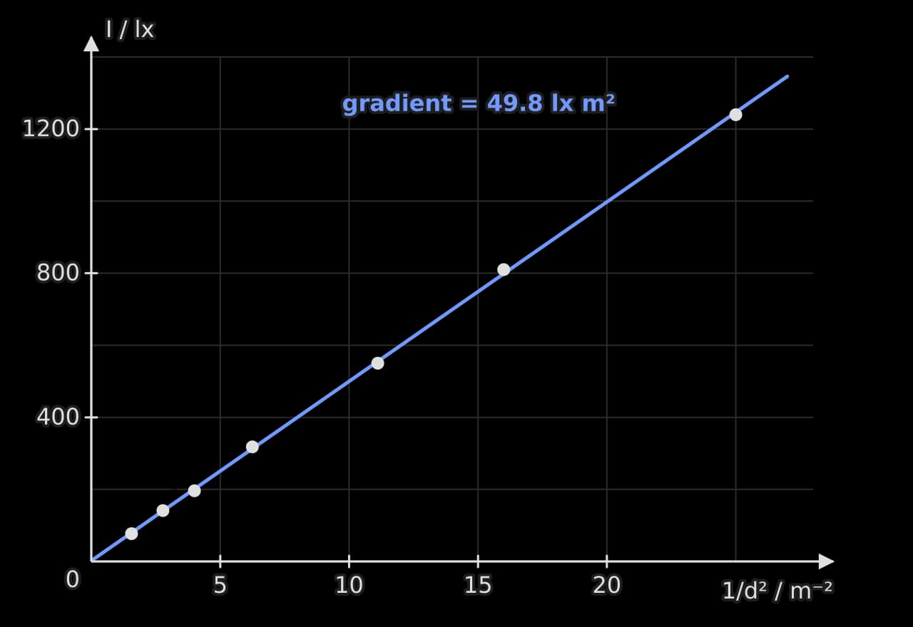
The points lie on a straight line through the origin (the intercept, 1.8 lx, is small compared with the readings), so the data support the inverse-square law over this range, and the gradient gives $k=49.8{\text{lx m}}^2$.

Log–log graphs for an unknown power

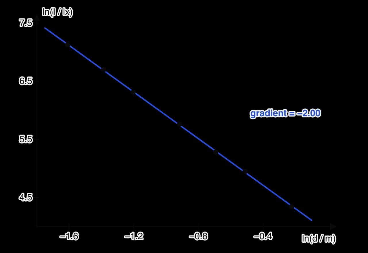
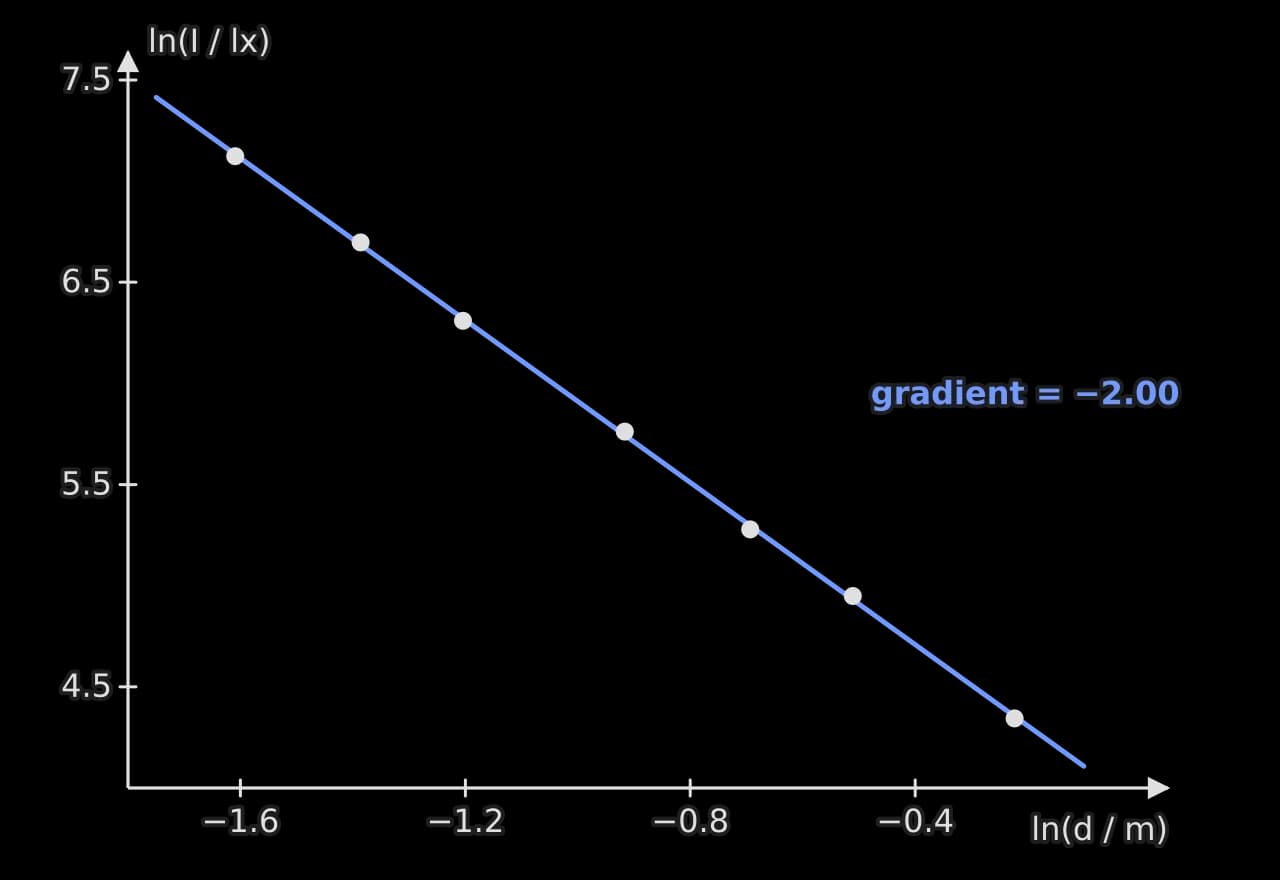
If theory gives $y=k{x}^n$ but the power $n$ is unknown (or is what the investigation is testing), taking logarithms of both sides gives

so a graph of $\ln y$ against $\ln x$ is a straight line with gradient $n$ and intercept $\ln k$. For the light data the gradient is −2.00, confirming the power. A log–log graph is the best first test when the form of a power law is in doubt, because a straight line on it shows that a power law holds at all, and the gradient gives the power.

A fully worked analysis

The worked analysis follows one sample data set from raw readings to a final value with its uncertainty: the resistivity of constantan wire. The data are illustrative, of the kind a student would obtain with the apparatus of a wire on a metre rule connected to a digital ohmmeter.

Research question and theory

How does the length of a 0.38 mm diameter constantan wire, from 0.100 m to 0.800 m, affect its resistance, and what is the resistivity of constantan? For a uniform wire, $R=\rho L\mathrm{/}A$, where $\rho$ is the resistivity. The leads and clip contacts add a constant resistance $R_0$, so the prediction is a straight line $R=(\rho \mathrm{/}A)L+R_0$ with gradient $\rho \mathrm{/}A$.

Raw data

Sample data. The clip was removed and replaced between trials, so the spread includes the variation in contact resistance. The diameter was measured with a micrometer at five points along the wire: 0.37, 0.38, 0.38, 0.39 and 0.38 mm (zero reading checked as 0.00 mm). With the clips touching, the resistance was 0.20 Ω.

Processing

Mean resistance and uncertainty. For $L=0.400$ m:

Half the range is larger than the ohmmeter's resolution (0.01 Ω), so the spread sets the uncertainty. The other lengths are processed the same way.

Diameter. The mean of the five readings is 0.38 mm and half the range is 0.01 mm, so $d=0.38\pm 0.01$ mm and $A=(1.13\pm 0.06)\times {10}^{-7}{\text{m}}^2$, as found in the area example.

Graph. The resistance graph plots mean $R$ against $L$ with error bars. All eight points lie within their error bars of the best-fit line, so the data support a linear relationship over the whole range. The gradient is $m=4.31\pm 0.16\mathrm{\Omega }{\text{m}}^{-1}$ (3.7%), and the intercept is $0.22\pm 0.07\mathrm{\Omega }$.

Resistivity. Since $m=\rho \mathrm{/}A$,

So $\rho =(4.9\pm 0.4)\times {10}^{-7}\mathrm{\Omega }\text{ m}$.

The analysis has answered both parts of the question: resistance increases linearly with length (with a constant offset), and the resistivity has been found with an honest uncertainty. The diameter contributes more than half of the final uncertainty, which the evaluation will discuss. The intercept, 0.22 ± 0.07 Ω, agrees with the 0.20 Ω measured with the clips touching, which supports the explanation that it is the resistance of the leads and contacts.

Applying the ideas

Choosing between two estimates of uncertainty, as in that example, is itself part of the analysis. The report states which was used and why.

Both forms test the same prediction. Choosing which quantity to put on each axis is a design decision that the report can justify in a sentence.

Self-check

• To do:

  I can record raw data in a table with quantities, units, uncertainties and consistent decimal places.

• To do:

  I can estimate the uncertainty of a reading and of a set of repeated readings.

• To do:

  I can identify an outlier and justify how it was treated.

• To do:

  I can propagate uncertainties through sums, differences, products, quotients and powers.

• To do:

  I can show a sample calculation and present processed data in a table.

• To do:

  I can draw a graph with labelled axes, error bars and a line of best fit.

• To do:

  I can find a gradient and intercept with uncertainties from maximum and minimum lines.

• To do:

  I can linearise a predicted relationship, including with a log–log graph for an unknown power.

• To do:

  I can carry an analysis through from raw data to a final value with its uncertainty.