Conclusion and evaluation

How to write a conclusion justified by the data and their uncertainties, compare results with accepted values and theory, and evaluate weaknesses by their impact with realistic improvements.

IB Physics
Internal assessment
SL and HL

15 min readLast reviewed 14 Oct 2026

The Conclusion and Evaluation criteria together carry half the marks for the investigation. The conclusion answers the research question and justifies the answer with the processed data, their uncertainties and the accepted science. The evaluation judges how far that answer can be trusted: which weaknesses and limitations affected the result, how much each one mattered, and what realistic changes would reduce their effect.

Both criteria depend on the analysis. A gradient with an uncertainty, an intercept that may or may not be zero, and a derived value that can be compared with a published one give the conclusion something precise to say and the evaluation something specific to explain. Without uncertainties, neither criterion can reach the top band.

What the criteria reward

Criterion	Middle band (3–4)	Top band (5–6)
Conclusion	A relevant conclusion is described but not fully consistent with the analysis; some relevant comparison with the accepted scientific context	A relevant conclusion is justified, fully consistent with the analysis, and justified through relevant comparison with the accepted scientific context
Evaluation	Specific methodological weaknesses or limitations are described, with relevant realistic improvements described	The relative impact of specific weaknesses or limitations is explained, with relevant realistic improvements explained

Two words carry most of the difference. In the conclusion, justified means every claim is backed by a number from the analysis and its uncertainty. In the evaluation, relative impact means the weaknesses are not just listed but ranked by how much each one changed the result.

Writing a justified conclusion

A conclusion opens by answering the research question directly, in one or two sentences. It then supports that answer with evidence from the processed data, and finally places it in the scientific context.

Answering the question

Name the relationship precisely. "Resistance increases linearly with length" or "the period is proportional to the square of the length", not "length affects resistance". Use proportional only for a straight line through the origin (within its uncertainty).
Quote the key result with its uncertainty and unit. "The gradient is 4.3 ± 0.2 Ω m⁻¹, giving a resistivity of (4.9 ± 0.4) × 10⁻⁷ Ω m."
State the range of validity. The conclusion holds over the range investigated; it may not hold beyond it.
Use cautious language. Data support or are consistent with a hypothesis; they never prove it.

Using the uncertainties as evidence

The uncertainties decide what the data can claim. If every error bar touches the best-fit straight line, the data are consistent with a linear relationship. If the intercept, with its uncertainty, includes zero, the data are consistent with direct proportionality; if it does not, a systematic offset is present and must be explained. If the maximum and minimum lines allow very different gradients, the conclusion must be more tentative.

Comparing with the accepted scientific context

The scientific context is the published knowledge the result can be tested against: a theory's prediction, an accepted value of a constant or a material property, or the findings of earlier studies. Every comparison is cited so that the reader can trace its source.

Percentage error and the uncertainty range

The simplest comparison is the percentage error between the experimental and literature values:

percentage error = \frac{∣ experimental - accepted ∣}{accepted} \times 100 %

A percentage error on its own says little. The decisive comparison is whether the accepted value lies within the uncertainty range of the experimental result. Three cases are possible.

Case	What it suggests	What the conclusion says
Accepted value inside the uncertainty range	The result is consistent with the accepted value; any difference can be explained by random uncertainty	The result agrees with the accepted value within its uncertainty
Accepted value outside the range	A systematic error, or an assumption of the theory that does not hold, has affected the result	The result does not agree; the direction of the difference points to the likely cause
Range very wide, so almost any value fits	The result agrees, but the test is weak	Agreement is noted, with the caveat that the uncertainty is too large for a strong test

Comparing the percentage error with the percentage uncertainty gives the same test in one line. In the resistivity analysis, the percentage error from the literature value of $4.9 \times 10^{- 7} Ω$ m is less than 1%, far smaller than the 9% uncertainty, so the result agrees. If the percentage error had been 15%, larger than the uncertainty, a systematic error would be indicated.

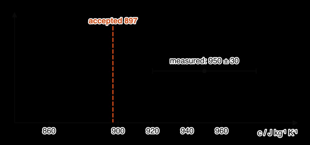
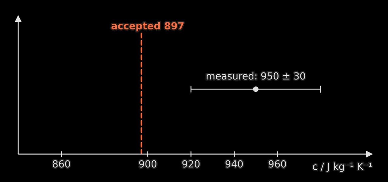
A horizontal scale of specific heat capacity from 840 to 1000 J kg⁻¹ K⁻¹. A measured value of 950 ± 30 is shown with an error bar from 920 to 980. An orange dashed vertical line marks the accepted value, 897, which lies outside the error bar. — Sample data. The accepted value (orange dashed line) lies outside the measured range of 920 to 980, so the random uncertainties alone cannot explain the difference: a systematic error is likely.

The comparison chart shows the second case for a specific heat capacity experiment. The measured value is 950 ± 30 J kg⁻¹ K⁻¹; the accepted value for aluminium near room temperature is about 897 J kg⁻¹ K⁻¹, below the lower limit of 920. The measured value is too high, and the direction of the difference is itself evidence: heat lost to the surroundings means more energy was supplied than the block absorbed, which makes the calculated $c$ too high.

Comparing with theory

When the research question tests a relationship rather than a value, the context is the theory's prediction. A log–log gradient of 1.95 ± 0.03 for a relationship predicted to have power 2 is close but does not include the predicted value, so either the theory's assumptions do not quite hold or a systematic error is present. A conclusion that explains which (with evidence, such as a non-zero intercept) is fully justified.

Weak and strong conclusions

The worked examples show how the same results support conclusions of very different quality.

A student measured the resistivity of constantan from the gradient of a graph of $R$ against $L$ , obtaining $(4.9 \pm 0.4) \times 10^{- 7} Ω$ m with an intercept of $0.22 \pm 0.07 Ω$ . Compare a weak and a strong conclusion.

Show the solution

Weak. "The results show that as the length of the wire increases, the resistance increases. This is because a longer wire has more resistance. The resistivity was 4.89 × 10⁻⁷ Ω m, which is very close to the real value, so the experiment was accurate."

The weak version gives no relationship type, no uncertainty, no source for the "real value", too many significant figures, and a circular explanation.

Strong. "Over the range 0.100 m to 0.800 m, the resistance of the constantan wire increases linearly with length: all eight points lie within their error bars of the best-fit line, $R = (4.3 \pm 0.2 Ω m^{- 1}) L + (0.22 \pm 0.07 Ω)$ . The relationship is not direct proportionality, because the intercept does not include zero; it agrees with the 0.20 Ω measured with the clips touching, so it is the resistance of the leads and contacts. This supports the model $R = ρ L / A + R_{0}$ . The resistivity from the gradient, $(4.9 \pm 0.4) \times 10^{- 7} Ω$ m, agrees with the literature value of $4.9 \times 10^{- 7} Ω$ m at 20 °C (Reference 3) within its 9% uncertainty."

The strong version could be checked line by line against the analysis, which is what "fully consistent with the analysis" means in practice.

A student's specific heat capacity experiment gives $c = 950 \pm 30$ J kg⁻¹ K⁻¹ for aluminium. Write a justified conclusion.

Show the solution

"The specific heat capacity of the aluminium block was found to be $950 \pm 30 {J kg}^{- 1} K^{- 1}$ . The accepted value for aluminium near room temperature is $897 {J kg}^{- 1} K^{- 1}$ (Reference 2), a percentage error of 6%, twice the 3% uncertainty. The accepted value lies outside the range 920–980, so the difference cannot be explained by the random uncertainties in the measurements. The measured value is too high, which is the direction expected if some of the electrical energy supplied was transferred to the surroundings rather than to the block. The result therefore does not agree with the accepted value, and the most likely cause is a systematic heat loss, assessed in the evaluation."

Evaluating the investigation

The evaluation examines the methodology critically: what was done well, what weakened the result, what limited the scope of the conclusion, and how each problem could be reduced. It concerns the investigation itself, so "human error" or "the equipment was not perfect" earn nothing. Every point is specific to this method and this data set.

Random and systematic errors

Errors fall into two kinds with different effects and different remedies.

	Random error	Systematic error
Effect on readings	Scatter above and below the true value	All readings shifted in the same direction
Effect on results	Reduces precision; widens error bars	Reduces accuracy; shifts a gradient or an intercept
Shown by	The spread of repeats and the scatter about the best-fit line	A non-zero intercept, or disagreement with the accepted value beyond the uncertainty
Reduced by	More repeats, averaging, a more sensitive instrument	Calibration, correcting zero errors, changing the method
Physics example	Reaction time when hand-timing; variable contact resistance	Heat loss in calorimetry; an unzeroed balance; lead resistance

A random error is reduced by repeating and averaging, but a systematic error is not: repeating a calorimetry experiment with the same heat loss gives the same wrong answer every time. A strong evaluation states which kind each weakness is, and therefore whether more repeats would help.

Explaining the relative impact

The top band asks for the relative impact of each weakness, which means ranking them. Two tools make this possible.

Percentage uncertainties. The contribution of each measurement to the final uncertainty shows which random uncertainties matter. In the resistivity analysis, the diameter contributes 5.3% and the gradient 3.7%, so the diameter is the largest single source.
Estimating a systematic effect. A systematic error can often be estimated from the data or from a short extra measurement. The size of the estimate is compared with the discrepancy it is meant to explain.

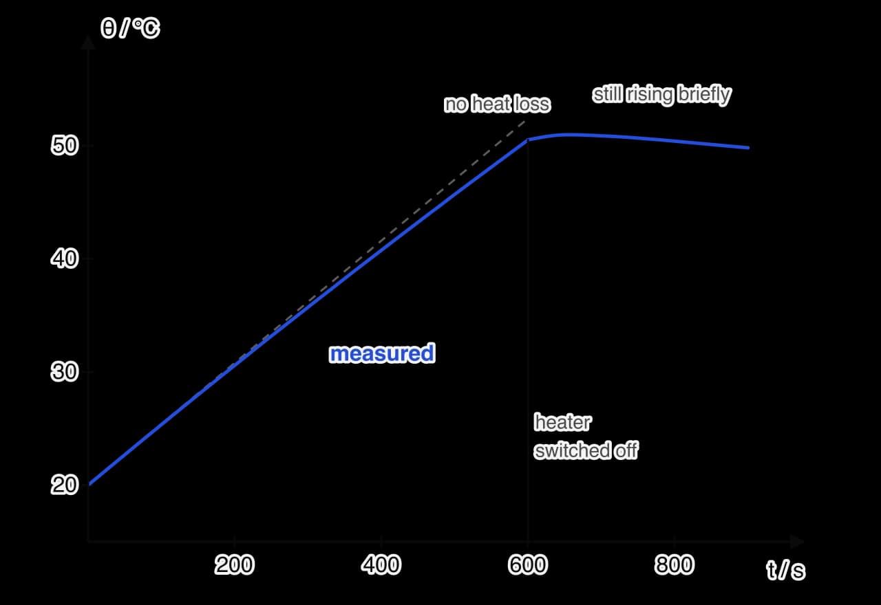
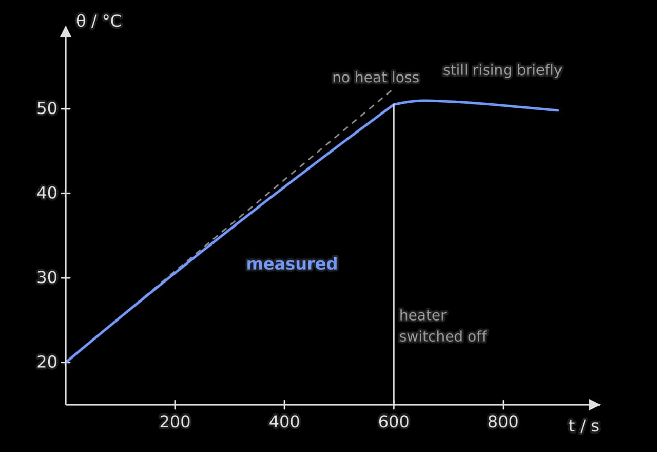
Graph of temperature against time for an aluminium block heated for 600 s. A dashed straight line rises from 20 °C to 52.4 °C, the prediction with no heat loss. — Sample data. Heat loss makes the measured curve (blue) bend below the no-loss line (dashed), and the temperature keeps rising briefly after switch-off while heat spreads from the heater.

The heating curve shows how a systematic heat loss can be estimated. After the heater was switched off, the 1.00 kg block cooled at about 0.37 K per minute at 50 °C, 30 K above room temperature. With $c \approx 900 {J kg}^{- 1} K^{- 1}$ that is a loss of about 5.6 W at the end of heating. The temperature excess rose roughly steadily from zero, so the average loss during heating was about half of that, 2.8 W, or about 1,700 J over 600 s. This is 6% of the 29,000 J supplied, which matches the 6% discrepancy. Heat loss is therefore large enough to explain most of the difference, and it is the dominant weakness.

Weak and strong evaluation points

Generic (lower band)	Specific and explained (top band)
"There was human error in timing."	"Hand-timing ten oscillations gave a spread of 0.14 s (1.9%). This random uncertainty is the largest contribution to the uncertainty of g; filming the oscillations at 240 frames per second would reduce it to about 0.01 s."
"More repeats would make it more accurate."	"The diameter varied by 0.02 mm along the wire, contributing 5.3% to the uncertainty in ρ, more than the gradient. Measuring the diameter at ten points rather than five, at different orientations, would reduce this; more resistance repeats would not, because they do not affect A."
"The equipment was not very precise."	"The ohmmeter's resolution (0.01 Ω) is small compared with the spread of repeats (up to 0.13 Ω), so the instrument was not limiting. The spread came from contact resistance at the sliding clip, which a four-terminal method would remove."
"Heat was lost."	"Heat loss of about 1,700 J (6% of the input), estimated from the cooling rate after switch-off, explains the measured value being 6% above the accepted value. Lagging the block with 2 cm of foam, or starting about 15 K below room temperature and finishing about 15 K above, would greatly reduce it."

Realistic improvements

Each improvement should be realistic (possible in a school laboratory in the time available), relevant (aimed at an identified weakness) and explained (saying how it would reduce the effect, ideally by how much). "Use a vacuum chamber" is rarely realistic; "use a light gate instead of a stopwatch, reducing the timing uncertainty from 0.2 s to 0.001 s" is.

Strengths, limitations and assumptions

A balanced evaluation also notes strengths: a wide range, small scatter, a method that removed an offset automatically. It considers limitations of scope, such as a conclusion valid only over the range tested or for one material, and the assumptions of the theory: was the wire really uniform, were the oscillations small enough for the simple model, was the source effectively a point? Where an assumption may have failed, the evaluation says how the data would show it.

A complete evaluation, weak and strong

Write an evaluation of the specific heat capacity experiment (1.00 kg aluminium block, a heater supplying about 48 W, 600 s, measured $c = 950 \pm 30$ J kg⁻¹ K⁻¹ against 897 J kg⁻¹ K⁻¹).

Show the solution

Weak version. "The experiment had some errors. Heat was lost to the surroundings and the thermometer might not have been accurate. There may have been human error reading the voltmeter. To improve, the experiment should be repeated more times and better equipment used."

Every point is generic, there is no ranking, and the improvements would not address the main problem.

Strong version.

Heat loss to the surroundings (systematic, dominant). From the cooling rate after switch-off, about 1,700 J (6% of the 29,000 J supplied) was lost during heating, comparable to the whole 6% excess, so this is the main cause. Improvement: wrap the block in 2 cm of expanded polystyrene, and start about 15 K below room temperature so that heat gained in the first half roughly cancels heat lost in the second.
Thermal lag (systematic, moderate). The temperature kept rising by about 0.45 K after switch-off. Using the switch-off reading rather than the maximum (50.95 °C) underestimated ΔT by about 1.5%, also making c too high. Improvement: record the maximum temperature after switch-off and use it for ΔT.
Thermal contact (systematic, small). Air gaps around the thermometer slow its response. Improvement: a drop of oil in the thermometer hole.
Random uncertainties (small). The largest are the current (1.2%) and pd (0.8%); with the temperature change they make up the 3% uncertainty. These are smaller than the systematic effects, so more repeats would not change the conclusion.

Strength. The electrical method measures the energy supplied directly and precisely, so the result depends mainly on the temperature measurements and heat loss, both of which can be estimated.

The strong version ranks the weaknesses, identifies their type and direction, and connects each improvement to the problem it solves. It uses about 300 words, which is a sensible share of a 3,000-word report.

Applying the ideas

That answer follows the pattern of every good comparison: inside or outside the range, the size of the disagreement against the uncertainty, the direction, and a cause that pushes in that direction.

Self-check

To do:
I can answer a research question directly, naming the relationship precisely.
To do:
I can use uncertainties and intercepts as evidence for or against a relationship.
To do:
I can compare a result with a traceable literature value using the uncertainty range.
To do:
I can explain what a disagreement and its direction suggest about systematic errors.
To do:
I can distinguish random and systematic errors and say which improvements reduce each.
To do:
I can rank weaknesses by their relative impact using numbers from my data.
To do:
I can suggest realistic, relevant improvements and explain how each would help.
To do:
I can include strengths, limitations of scope and assumptions in an evaluation.

Carry on with Physics in Augment

With a free account, Augment remembers where you stopped in the notes and which questions you have marked.

Start free