A complete investigation, start to finish

One investigation followed from first idea to evaluation: how the period of a vibrating steel rule depends on its length, with the data, graphs, conclusion and evaluation.

IB Physics
Internal assessment
SL and HL

16 min readLast reviewed 14 Oct 2026

This worked investigation follows one question through every stage: choosing and refining it, the theory, the method, the raw and processed data, the graphs, the conclusion and the evaluation. Each stage is annotated with the reasons behind its choices, which is what the criteria reward. The question is how the period of a steel rule clamped at one end and vibrating freely, a cantilever, depends on the length that overhangs the bench.

A vibrating rule is familiar from any classroom, where flicking a ruler over the edge of a desk makes a buzzing sound whose pitch rises as the overhang shortens. Behind it is a strong prediction from the theory of bending beams, and a material constant, the Young modulus of steel, that can be found from the results and checked against published values.

From an idea to a research question

The idea began with the buzzing ruler. The first version of the question, "How does the length of a ruler affect the sound it makes?", is too vague: "sound" could mean loudness, pitch or duration, and a plastic ruler slapping on the desk makes a noise unrelated to its vibration.

One relationship. The frequency (or period) of free vibration as a function of the overhanging length.
A better system. A stainless steel rule, which vibrates for many cycles and has well-known elastic properties, held in a G-clamp so that it does not slap on the bench.
A measurable dependent variable. Measuring pitch by ear is imprecise, and a phone microphone picks up the bench's own vibrations. Filming the tip at 240 frames per second and counting frames gives the period directly.
A prediction. Beam theory predicts that the period is proportional to the square of the length.

What the pilot showed

A pilot run at three lengths, 0.10 m, 0.30 m and 0.50 m, decided the range.

At 0.10 m the frequency was about 60 Hz, so each cycle lasted only about four video frames, too few to identify each oscillation reliably. The shortest usable length was 0.15 m, about eight frames per cycle.
At 0.50 m only 0.10 m of the 0.60 m rule remained under the clamp, and the rule rocked visibly in the clamp. The longest secure length was 0.45 m, leaving 0.15 m clamped.
Repeat counts at one length differed by at most two frames, so three repeats were enough to estimate the scatter.
At short lengths one period is so brief that counting 20 oscillations kept the counting uncertainty small; at longer lengths the oscillation decayed noticeably after about 15 cycles, so 10 were counted.

Research question. How does the overhanging length of a clamped stainless steel rule, from 0.150 m to 0.450 m, affect the period of its free vibration, and is the period proportional to the square of the length, as cantilever theory predicts, with a gradient that gives the Young modulus of the steel?

Background theory

A thin, uniform beam clamped at one end vibrates in a set of modes, like a string. In its first mode the whole overhang swings to and fro with the tip moving most. The theory of bending beams (Euler–Bernoulli theory, Reference 1) gives the frequency of the first mode as

f = \frac{3.516}{2 π L^{2}} \sqrt{\frac{E I}{μ}}

where $L$ is the overhanging length, $E$ the Young modulus of the material (its stiffness, in Pa), $I$ the second moment of area of the cross-section (in $m^{4}$ , a measure of how the cross-section resists bending), and $μ$ the mass per unit length (in ${kg m}^{- 1}$ ). The constant 3.516 comes from the solution of the beam equation for the first mode. For a rectangular cross-section of width $w$ and thickness $d$ , $I = w d^{3} / 12$ . The period is $T = 1 / f$ , so

T = \frac{2 π}{3.516} \sqrt{\frac{μ}{E I}} L^{2}

This predicts that $T \propto L^{2}$ . A graph of $\ln T$ against $\ln L$ should therefore have a gradient of 2, and a graph of $T$ against $L^{2}$ should be a straight line through the origin with gradient

k = \frac{2 π}{3.516} \sqrt{\frac{μ}{E I}} ⟹ E = {(\frac{2 π}{3.516})}^{2} \frac{μ}{I k^{2}}

The model assumes that the rule is uniform, that the clamp holds it perfectly rigidly at the clamp edge, that the amplitude is small, and that the air has a negligible effect on the motion. Each of these assumptions will be examined in the evaluation.

The Young modulus of type 304 stainless steel, a common material for steel rules, is given in manufacturers' data sheets as about 193–200 GPa (Reference 2).

Variables and method

Variable	Type	How it is set, measured or controlled	Why
Overhang $L$	Independent	0.150 to 0.450 m in steps of 0.050 m, measured with a metre rule from the clamp edge to the tip; ± 0.002 m	Seven values over the full usable range (from the pilot)
Period $T$	Dependent	Frames counted for 20 (short $L$ ) or 10 (long $L$ ) oscillations at 240 frames per second; three repeats	Counting many cycles reduces the uncertainty per period
Amplitude	Control	Tip displaced 10 mm against a pointer and released	Large amplitudes change the period slightly and make the rule rattle in the clamp
Clamping	Control	Same steel block and G-clamp, tightened fully each time; the block's edge aligned with the bench edge	A loose clamp lengthens the effective vibrating length
The rule	Control	The same 600 mm rule, its scale face up	μ, w, d and E must be the same for every length
Temperature	Control (monitored)	21 ± 1 °C in the laboratory	E changes very little over this range

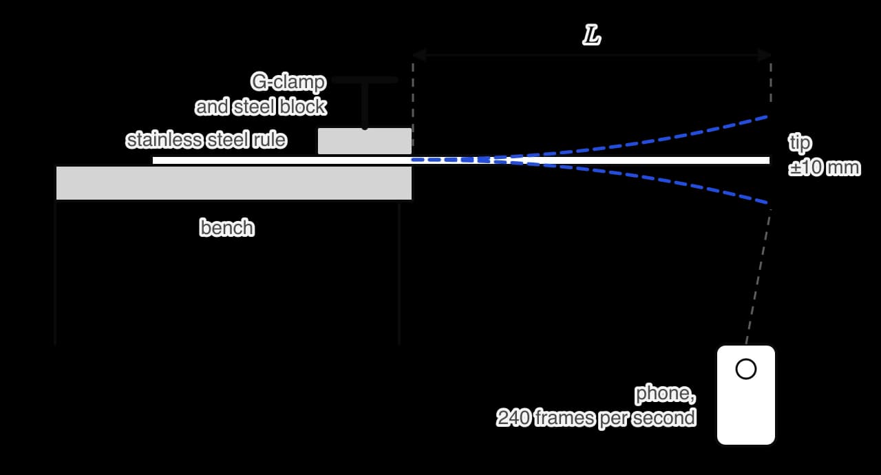
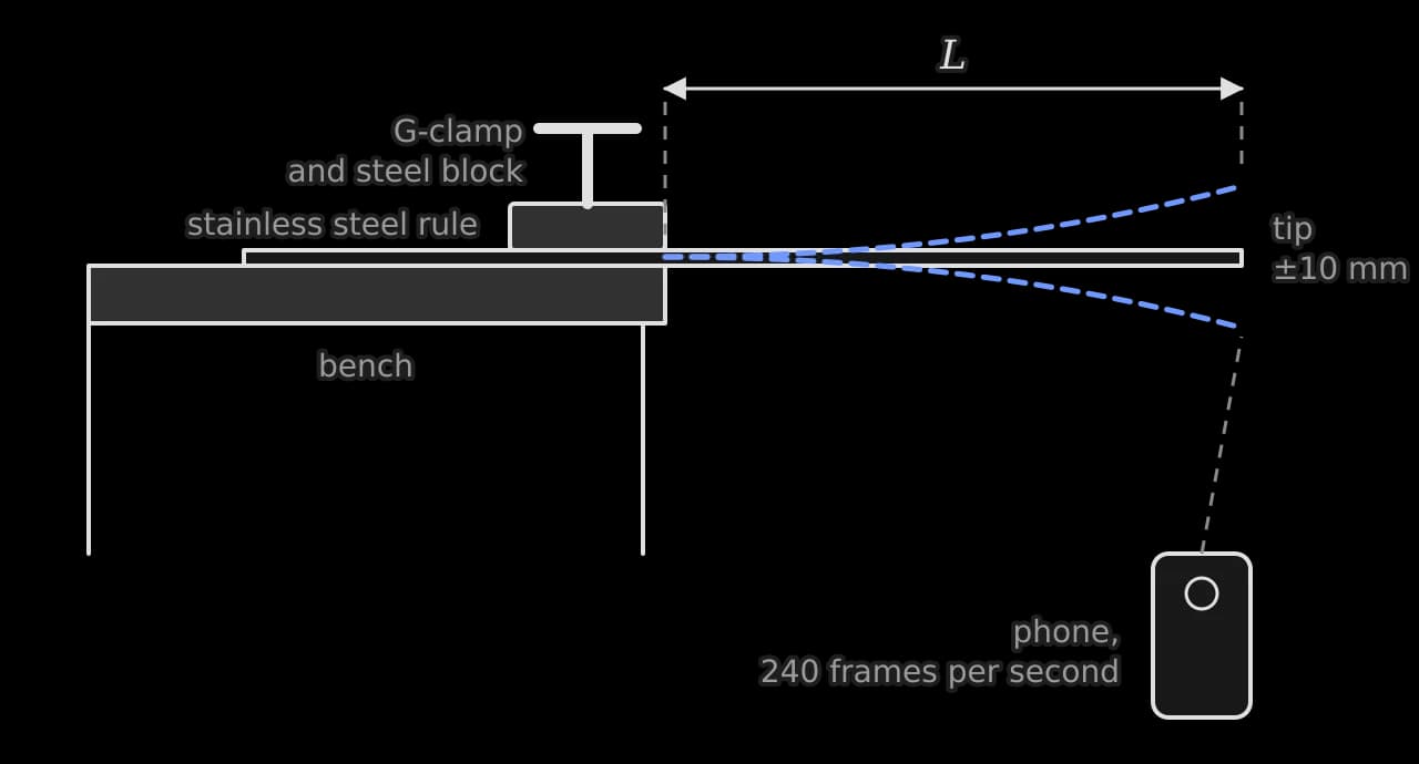
Side view: a stainless steel rule lies on a bench, held at the bench edge by a steel block pressed down by a G-clamp, with length L overhanging. Blue dashed curves show the rule bent up and down as it vibrates. A phone in front of the tip, below the bench top, films it at 240 frames per second. — The vibrating length L runs from the edge of the clamping block to the tip. The tip is displaced 10 mm and released, and the phone films the oscillation from the side.

Procedure

Measure the mass of the rule on a top-pan balance (0.1 g resolution), its length with a metre rule, its width with vernier calipers at five points, and its thickness with a micrometer at five points.
Clamp the rule to the bench with the steel block's edge at the bench edge, set $L = 0.150$ m, and tighten the G-clamp fully.
Set the phone on a stand 30 cm in front of the tip, with a pointer marking the tip's rest position, and start recording at 240 frames per second.
Push the tip down 10 mm to the pointer and release it.
In the video, find the frame where the tip first passes the rest position moving upwards, then count frames until it has completed 20 (or 10) further oscillations.
Repeat steps 4 and 5 twice more, then repeat for each length.

Safety. The tip of a steel rule has sharp corners and can flick up when released; eye protection is worn and the face kept above the clamped end. The G-clamp is checked for security before each release. There are no ethical issues, and no materials are used up.

Raw data

The measurements of the rule itself were: mass 106.7 ± 0.1 g, length 0.600 ± 0.001 m, width 25.0 ± 0.1 mm (five readings within 0.1 mm), thickness 0.90 ± 0.01 mm (five readings from 0.89 to 0.91 mm).

$L$ / m ± 0.002	Oscillations counted $N$	Frames, trial 1 ± 2	Frames, trial 2 ± 2	Frames, trial 3 ± 2
0.150	20	164	161	163
0.200	20	282	285	284
0.250	20	440	438	436
0.300	10	312	314	313
0.350	10	424	422	425
0.400	10	551	553	550
0.450	10	692	695	694

Sample data. The uncertainty of ± 2 frames per count comes from judging the start and end frames. The tip moved cleanly with no visible rattle at any length.

Processing

Period and its uncertainty

Sample calculation for $L = 0.300$ m. The mean count is $(312 + 314 + 313) / 3 = 313.0$ frames. Half the range is 1 frame, smaller than the reading uncertainty of 2 frames, so ± 2 frames is used. Each frame lasts $1 / 240$ s, and 10 oscillations were counted:

\begin{aligned} T & = \frac{313.0}{240 \times 10} = 0.1304 s \\ Δ T & = \frac{2}{240 \times 10} = 0.0008 s \end{aligned}

$L$ / m ± 0.002	$T$ / s	$Δ T$ / s	$L^{2}$ / m²	$Δ (L^{2})$ / m²	$\ln (L / m)$	$\ln (T / s)$
0.150	0.0339	0.0004	0.0225	0.0006	−1.897	−3.384
0.200	0.0591	0.0004	0.0400	0.0008	−1.609	−2.829
0.250	0.0912	0.0004	0.0625	0.0010	−1.386	−2.395
0.300	0.1304	0.0008	0.0900	0.0012	−1.204	−2.037
0.350	0.1765	0.0008	0.1225	0.0014	−1.050	−1.734
0.400	0.2297	0.0008	0.1600	0.0016	−0.916	−1.471
0.450	0.2890	0.0008	0.2025	0.0018	−0.799	−1.241

The uncertainty in $L^{2}$ is $2 (Δ L / L) \times L^{2}$ ; for $L = 0.300$ m it is $2 \times (0.002 / 0.300) \times 0.0900 = 0.0012 m^{2}$ . The percentage uncertainty in $T$ is between 0.3% and 1.2%, while that in $L^{2}$ is between 0.9% and 2.7%, so the length measurement is the larger source of random uncertainty.

Testing the power law

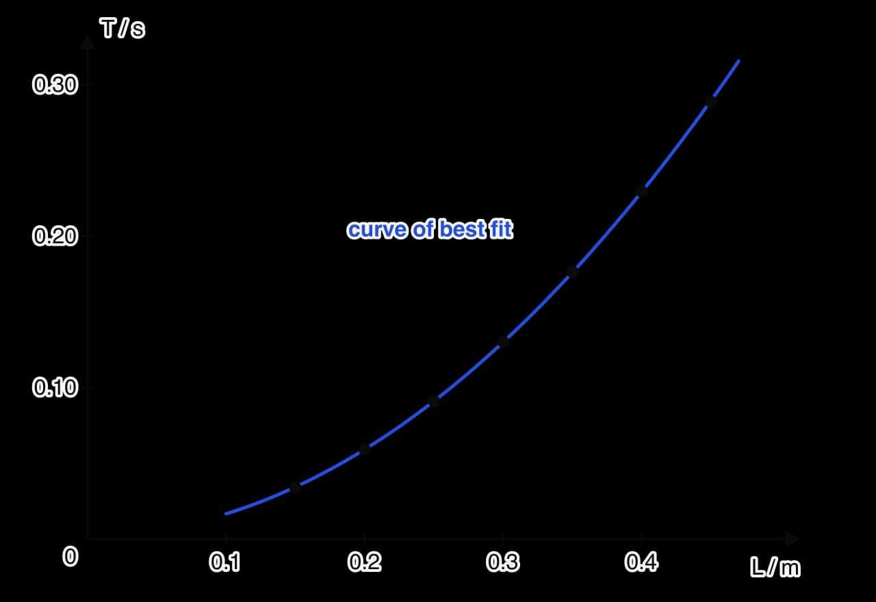
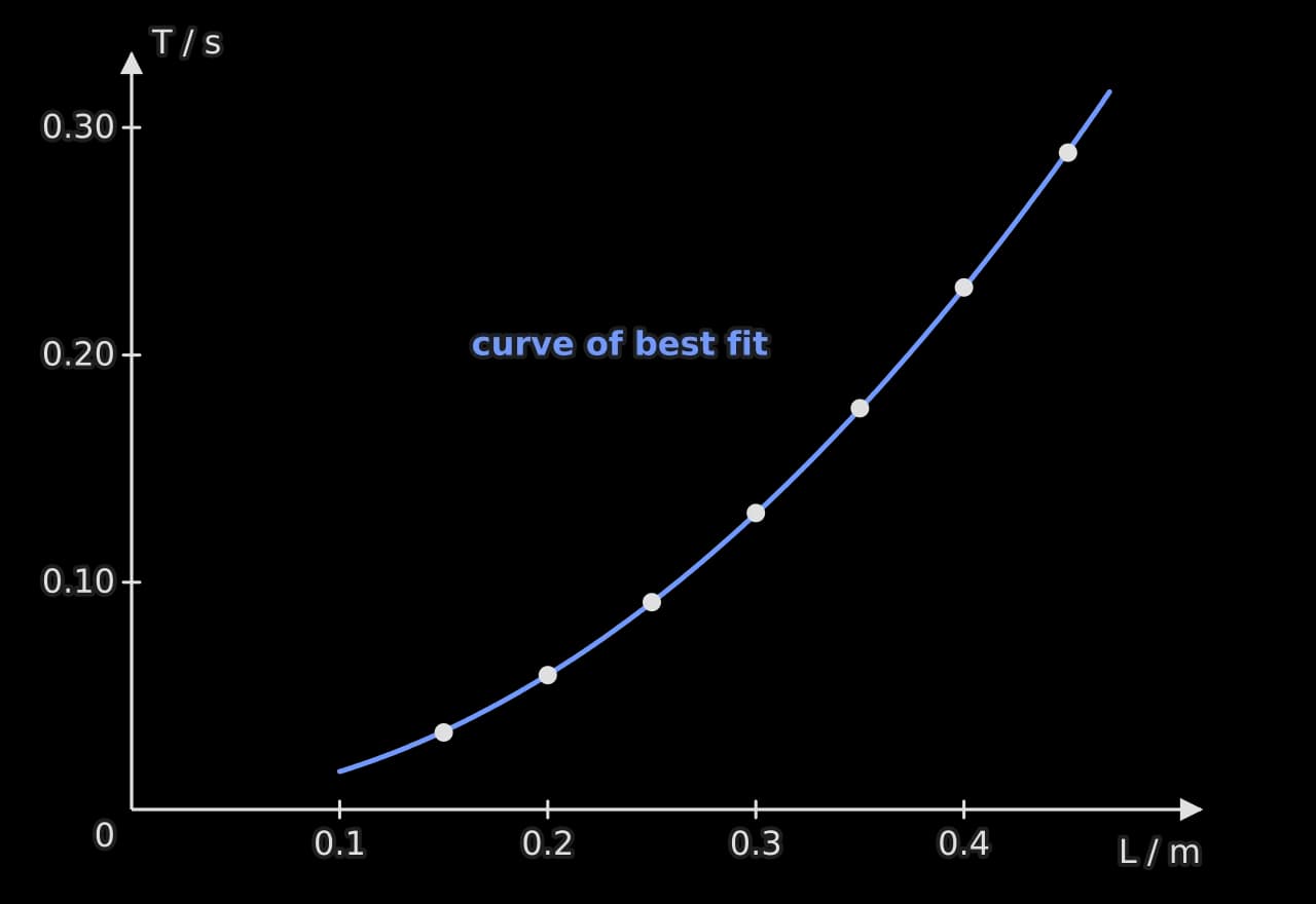
Graph of period T in seconds against overhang length L in metres. Seven points rise from 0.034 s at 0.15 m to 0.289 s at 0.45 m along a blue curve that gets steeper as L increases. — Sample data. The period rises more and more steeply with length, as a power law with a power greater than 1 would. Error bars are smaller than the dots.

The direct graph of period against length is a curve, so its shape alone cannot test $T \propto L^{2}$ . A log–log graph tests the power directly.

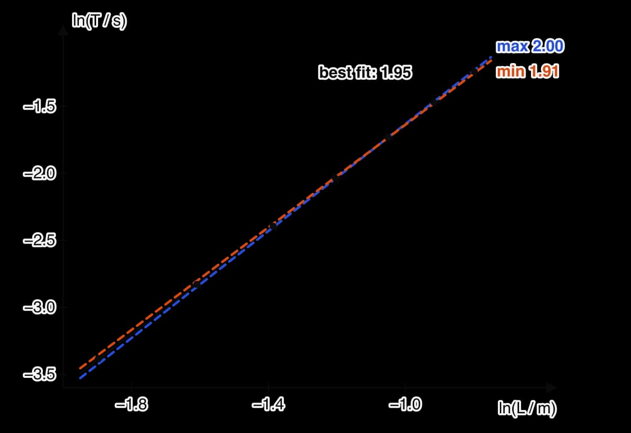
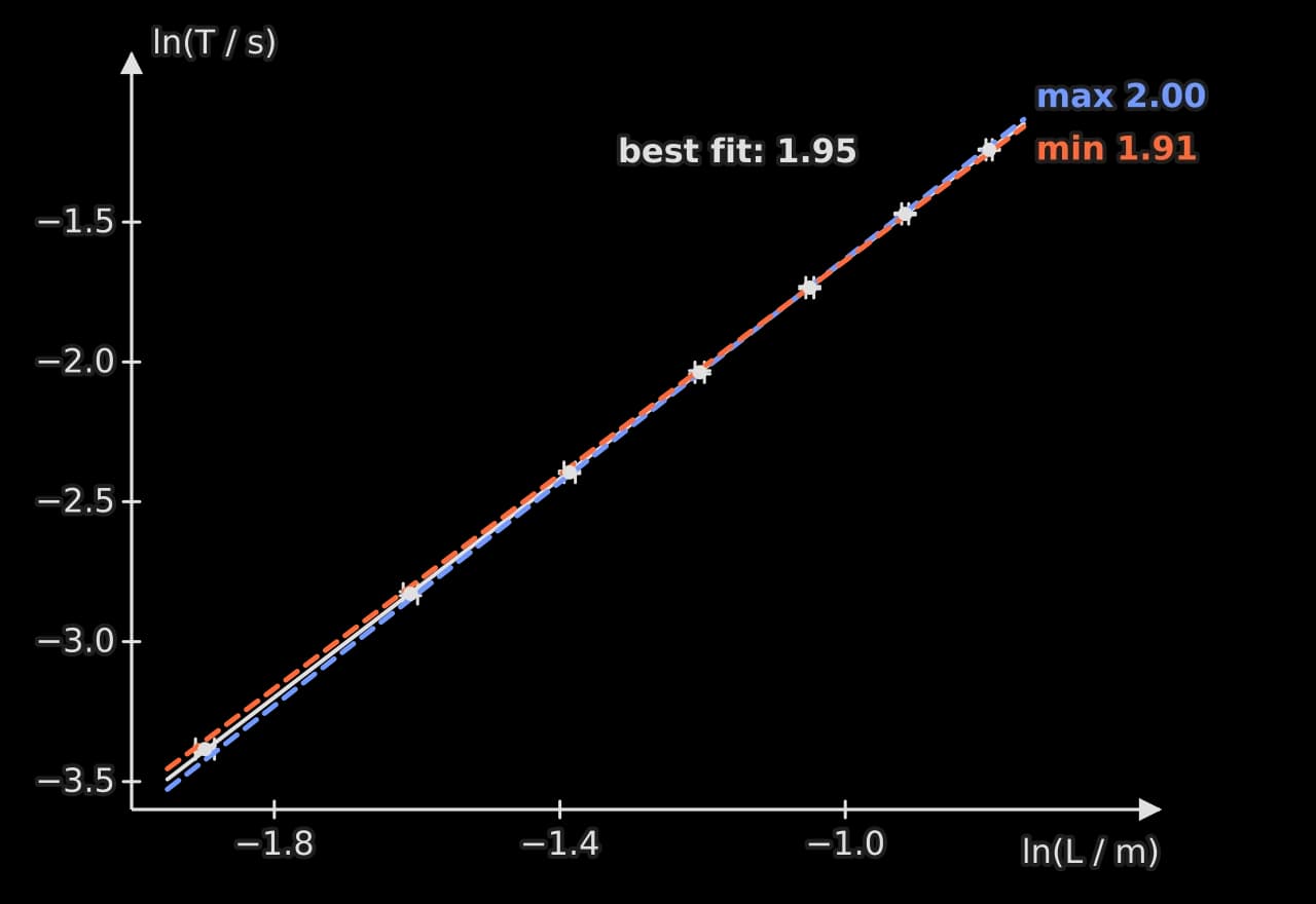
Graph of ln(T / s) against ln(L / m). Seven points with small error bars lie on a straight best-fit line of gradient 1.95, from about (−1.90, −3.38) to (−0.80, −1.24). A blue dashed maximum line has gradient 2.00 and an orange dashed minimum line 1.91. — Sample data. The straight line confirms a power law. Its gradient, 1.95 ± 0.04, is close to the predicted 2, which lies just at the top of the range.

The log–log graph is a straight line, so the data follow a power law. The best-fit gradient is 1.953, and the steepest and shallowest lines through all the error bars have gradients 1.996 and 1.913, so the power is $n = 1.95 \pm 0.04$ . The predicted value, 2, lies at the very top of this range.

Finding the Young modulus

Taking the predicted power of 2, a graph of $T$ against $L^{2}$ gives the constant $k$ .

Graph of period T in seconds against L squared in square metres from 0 to 0.22. Seven points with small horizontal error bars lie on a straight best-fit line of gradient 1.418 s m⁻² and a small positive intercept. — Sample data, linearised. T against L² is a straight line, as predicted; the gradient gives Young's modulus. The intercept, 0.0025 s, is small but positive.

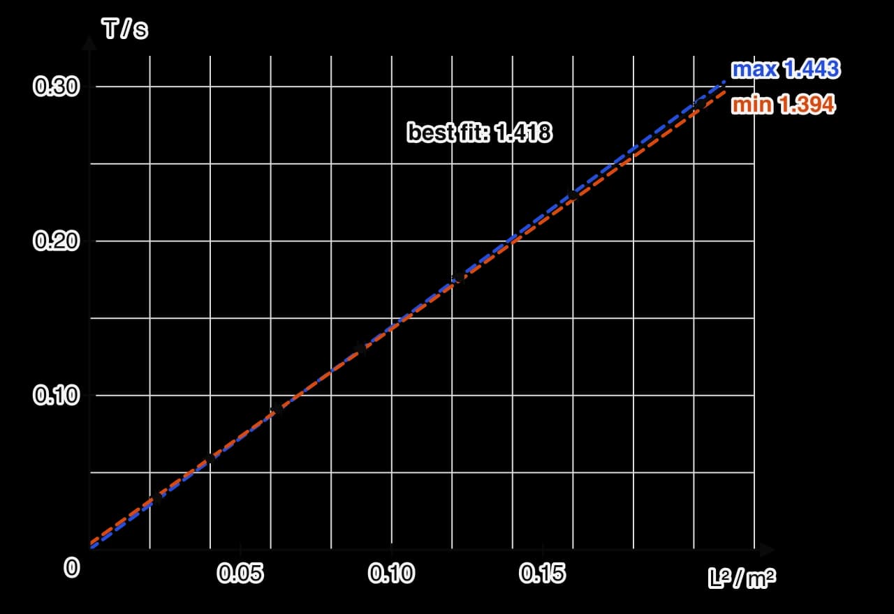
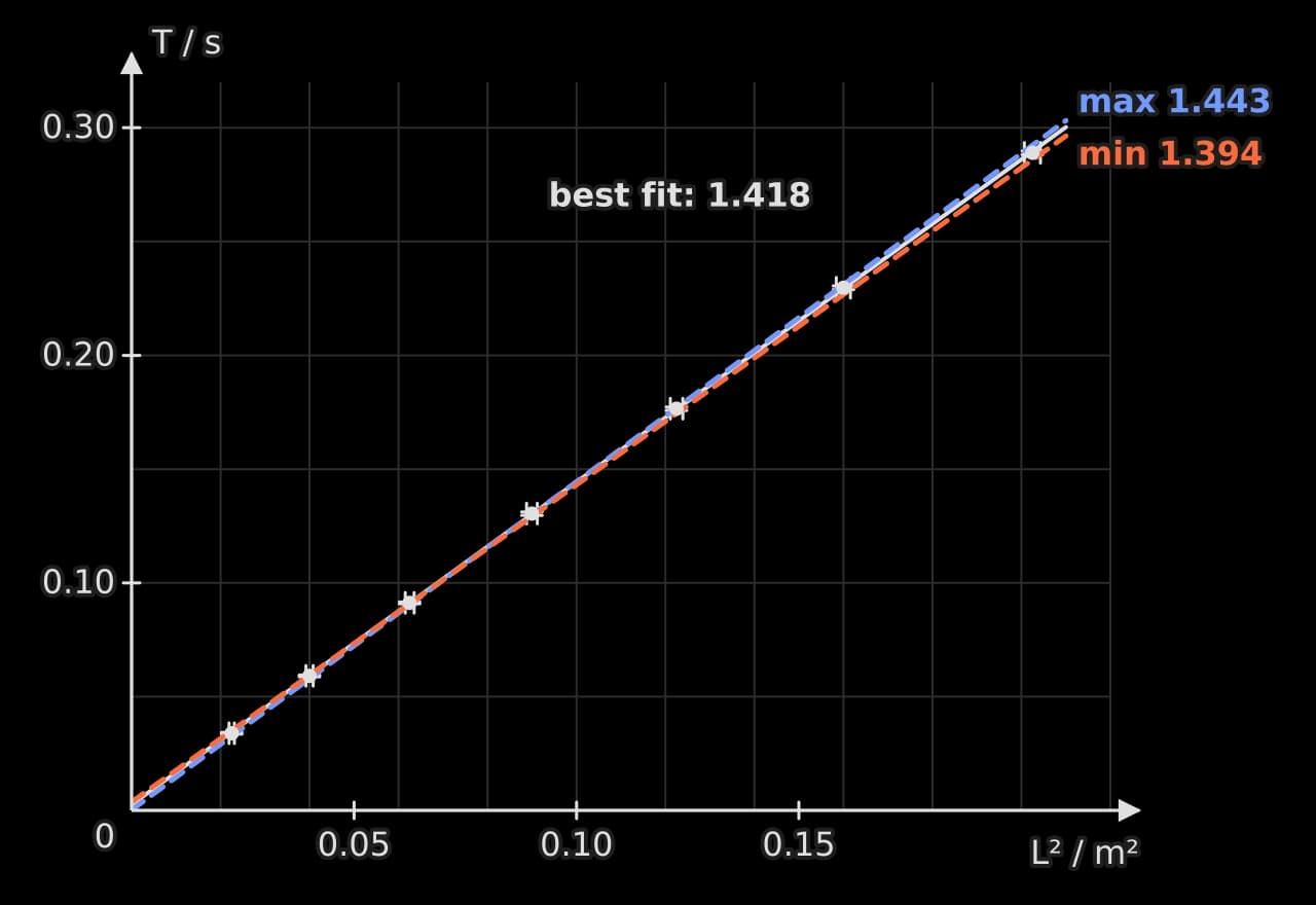
The gradient of the best-fit line is $k = 1.418 {s m}^{- 2}$ , with maximum and minimum gradients of $1.443$ and $1.394 {s m}^{- 2}$ , so $k = 1.418 \pm 0.025 {s m}^{- 2}$ (1.8%). The intercept is $0.0025 \pm 0.0018$ s: small, but positive even at the lower limit.

Mass per unit length and second moment of area.

\begin{aligned} μ & = \frac{0.1067}{0.600} = 0.1778 {kg m}^{- 1} (\pm 0.3 %) \\ I & = \frac{w d^{3}}{12} = \frac{0.0250 \times (0.90 \times 10^{- 3})^{3}}{12} = 1.519 \times 10^{- 12} m^{4} \\ \frac{Δ I}{I} & = \frac{0.1}{25.0} + 3 \times \frac{0.01}{0.90} = 0.4 % + 3.3 % = 3.7 % \end{aligned}

Young modulus.

\begin{aligned} E & = {(\frac{2 π}{3.516})}^{2} \frac{μ}{I k^{2}} = 3.193 \times \frac{0.1778}{1.519 \times 10^{- 12} \times {1.418}^{2}} = 1.86 \times 10^{11} Pa \\ \frac{Δ E}{E} & = \frac{Δ μ}{μ} + \frac{Δ I}{I} + 2 \frac{Δ k}{k} = 0.3 % + 3.7 % + 3.5 % = 7.5 % \\ Δ E & = 0.075 \times 1.86 \times 10^{11} = 0.14 \times 10^{11} Pa \end{aligned}

So $E = (1.86 \pm 0.14) \times 10^{11}$ Pa.

Conclusion

Over the range 0.150 m to 0.450 m, the period of the clamped steel rule increases as a power of the overhanging length: the log–log graph is straight, with gradient $1.95 \pm 0.04$ . This is consistent with the cantilever prediction $T \propto L^{2}$ , although the predicted power lies only at the top of the uncertainty range. The graph of $T$ against $L^{2}$ is a straight line with gradient $1.418 \pm 0.025 {s m}^{- 2}$ , giving a Young modulus of $(1.86 \pm 0.14) \times 10^{11}$ Pa.

The published Young modulus of type 304 stainless steel is 193–200 GPa (Reference 2). The measured value is 3.6% below 193 GPa, and its range, 172–200 GPa, includes the whole published range, so the result agrees with the accepted value within its 7.5% uncertainty.

Two features of the data point the same way. The power is slightly below 2, and the $T$ against $L^{2}$ line has a positive intercept that does not include zero. Both are what would happen if the true vibrating length were slightly longer than the measured $L$ by a constant amount, as it would be if the rule could flex a little inside the clamp. That would make every period slightly too long for its measured length, most noticeably at short lengths, and would make $k$ too large and $E$ too small. The measured $E$ is indeed at the low end of the accepted range, so the result is consistent with a small systematic effect from the clamp.

Evaluation

Strengths

Filming at 240 frames per second and counting 10 or 20 oscillations gave periods with uncertainties of 1.2% or less, far smaller than hand-timing could achieve for periods of 0.03 to 0.3 s.
The range covered the whole usable length of the rule, a factor of 3 in $L$ and 9 in $L^{2}$ , enough to test the power law clearly.
Using the gradient rather than a single length removed any constant offset in $T$ from the value of $E$ .

Weaknesses and limitations, in order of impact

Flexing of the rule inside the clamp (systematic, largest effect on accuracy). The positive intercept and the power slightly below 2 both suggest an effective length longer than $L$ . A graph of $\sqrt{T}$ against $L$ (which is linear if $T = k (L + δ)^{2}$ ) has an intercept on the $L$ axis at $- δ$ and gives $δ \approx 6$ mm, although with an uncertainty of about ± 6 mm. Repeating the analysis with $L + 6$ mm in place of $L$ gives $k = 1.39 {s m}^{- 2}$ and $E \approx 1.94 \times 10^{11}$ Pa, within the accepted range. The correction is suggestive rather than conclusive because $δ$ is so uncertain. Improvement: clamp the rule between two machined steel blocks the full width of the rule, bolted together, so that it cannot flex inside the clamp; or test the clamp directly by measuring the period at one fixed $L$ with the clamp tightened to two different forces, which would differ if the rule flexes inside it.
Thickness of the rule (random, largest contribution to the uncertainty in E). The thickness appears cubed in $I$ , so its 1.1% uncertainty contributes 3.3% to $E$ , nearly half of the 7.5% total. Improvement: measure the thickness at ten or more points along the vibrating part only, with a micrometer that reads to 0.001 mm, which would reduce this contribution below 1%.
Gradient of the graph (random, second largest contribution). The 1.8% uncertainty in $k$ contributes 3.5% to $E$ . It comes mainly from the uncertainty in $L$ (±2 mm, set by judging the clamp edge). Improvement: mark the clamp edge on the rule with a fine scribed line and measure $L$ with vernier calipers against it, reducing $Δ L$ to about 0.5 mm.
Assumption of small amplitude and negligible air effects (limitation). A tip displacement of 10 mm on a 0.15 m overhang is a deflection of about 7%. Fluid resistance from the air damps the motion, as the decay after about 15 cycles showed, and damping lengthens the period very slightly. Improvement: repeat one length at amplitudes of 5, 10 and 20 mm to check that the period does not depend on amplitude.
Range of the conclusion (limitation). The result applies to one rule of one material over 0.15–0.45 m. A thicker rule or a different metal would test whether $T \propto L^{2}$ holds generally, and a second rule of known material would check the method.

The square-root check of the clamp effect

If the true vibrating length is $L + δ$ , then $T = k (L + δ)^{2}$ and $\sqrt{T} = \sqrt{k} L + \sqrt{k} δ$ . A graph of $\sqrt{T}$ against $L$ is a straight line with gradient $\sqrt{k}$ and intercept $\sqrt{k} δ$ , so $δ$ = intercept ÷ gradient. For the sample data the gradient is $1.179 s^{1 / 2} m^{- 1}$ and the intercept $0.0073 s^{1 / 2}$ , so $δ \approx 0.0062$ m. The intercept's uncertainty (from maximum and minimum lines) is about ±0.007, so $δ$ is only known to about ±6 mm.

The gradient gives $k = {1.179}^{2} = 1.390 {s m}^{- 2}$ , which would give $E = 1.94 \times 10^{11}$ Pa. The check is useful because it uses the same data to test a specific explanation for the intercept, but it cannot replace a better clamp.

How the investigation meets the criteria

Criterion	Where this investigation earns the top band
Research design	A focused question with a range and prediction; a specific context from beam theory with its assumptions; methodological choices explained from the pilot (the 0.15 m and 0.45 m limits, 20 or 10 oscillations, three repeats); a repeatable procedure with a labelled diagram; safety addressed
Data analysis	Raw data with units, uncertainties and consistent precision; one sample calculation of each type; uncertainties propagated into $T$ , $L^{2}$ , $I$ and $E$ ; a log–log test of the power; a linearised graph with error bars and maximum and minimum lines
Conclusion	Answers both parts of the question with numbers and uncertainties; compares $E$ with a referenced accepted range; uses the power and the intercept as evidence of a systematic effect, with its direction
Evaluation	Strengths; weaknesses ranked by their effect, each classified as systematic or random, with numbers; the clamp effect estimated from the data; realistic, specific improvements explained

The investigation used only a steel rule, a G-clamp, a balance, a micrometer, vernier calipers and a phone. What makes it strong is the reasoning recorded at every step, from the choice of range to the ranking of the weaknesses.

Self-check

To do:
I can refine a first idea into a focused research question with a range and a prediction.
To do:
I can use a pilot to set the range, the number of oscillations and the number of repeats.
To do:
I can write the background theory for a prediction, including its assumptions.
To do:
I can process frame counts into periods with uncertainties.
To do:
I can test a power law with a log–log graph and find the power with its uncertainty.
To do:
I can find a constant from the gradient of a linearised graph and propagate its uncertainty.
To do:
I can write a conclusion that compares a result with a referenced accepted value.
To do:
I can rank weaknesses by their impact and use the data to estimate a systematic effect.

Carry on with Physics in Augment

With a free account, Augment remembers where you stopped in the notes and which questions you have marked.

Start free