Uncertainties and graphs

Random and systematic errors, accuracy and precision, absolute, fractional and percentage uncertainties and how they propagate, error bars, best-fit and max/min gradient lines, and linearising data, including logarithmic plots.

IB Physics
Exam skills
SL and HL

26 min readLast reviewed 14 Oct 2026

No measurement is exact. A length read from a rule, a time from a stopwatch or a current from an ammeter is always uncertain by some amount, and any quantity calculated from these readings inherits that uncertainty. Quoting a result with its uncertainty says how far it can be trusted, and it is what allows two results, or a result and a theory, to be compared fairly.

Graphs are the main tool for turning many uncertain readings into one reliable result. A well-drawn graph averages out random scatter, shows whether a relationship has the form a theory predicts, and gives a constant, with its uncertainty, from its gradient or intercept. These skills are tested throughout Paper 1B and are central to the internal assessment.

Key points

Random errors scatter readings on both sides of the true value and are reduced by repeating; systematic errors shift every reading the same way and are not.
Precision describes how closely readings agree; accuracy describes how close they are to the true value.
Uncertainties are written as absolute, fractional or percentage values, to one significant figure.
Absolute uncertainties add for sums and differences; fractional uncertainties add for products and quotients and are multiplied by the power for powers.
Error bars show the absolute uncertainty of each point. The steepest and shallowest lines through all of them give the uncertainty in the gradient and intercept.
A relationship is linearised by plotting quantities that the theory predicts are in a straight-line relation; logarithms find an unknown power.

Errors and uncertainties

In physics an error is not a mistake. It is the difference between a measured value and the true value, which can never be known exactly. The uncertainty is the range within which the true value is expected to lie, and it is what can actually be estimated from an experiment. A length recorded as $(24.6 \pm 0.1)$ cm means the true length is expected to lie between 24.5 and 24.7 cm.

Errors come in two kinds, which behave differently and are dealt with differently.

Random errors

Random errors arise from the limited resolution of an instrument, from small fluctuations in conditions (draughts, vibrations, electrical noise), and from human judgement, such as deciding exactly when a pendulum passes a marker. Because they are equally likely to make a reading too big or too small, averaging several readings tends to cancel them. Measuring a larger quantity, such as 20 oscillations instead of one, also makes their effect relatively smaller.

Systematic errors

Typical sources are an instrument that is wrongly calibrated, a zero error (an instrument that does not read zero when it should, such as a balance showing 0.3 g with nothing on it), reading a scale from the same wrong angle every time (parallax), and a feature of the method itself, such as energy lost to the surroundings in a heating experiment, which always makes a calculated specific heat capacity too large.

A systematic error can be hard to notice, because the readings agree well with each other. It shows up when a result is compared with an accepted value, or on a graph, where a line that should pass through the origin misses it. A zero error in the dependent variable moves the line up or down without changing its gradient.

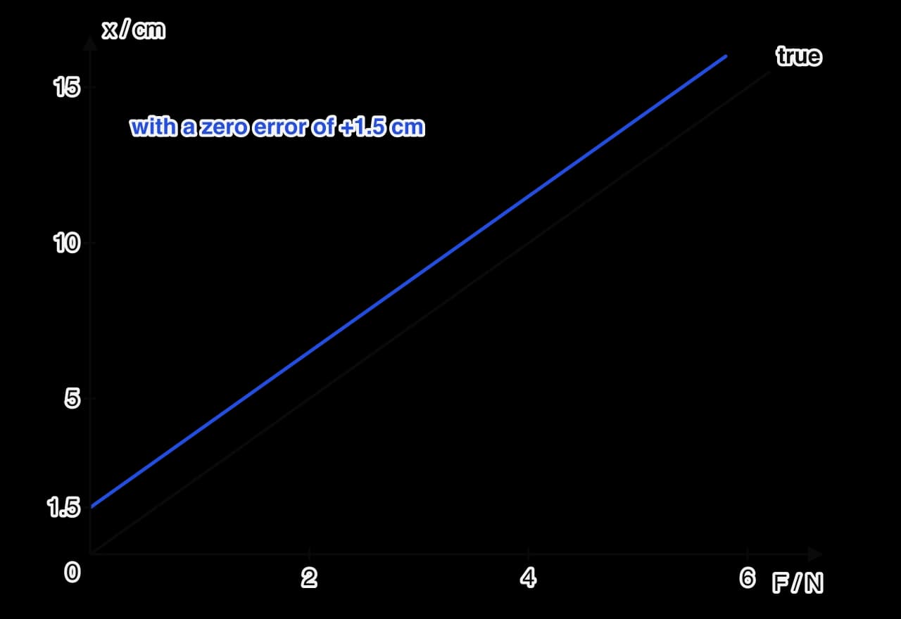
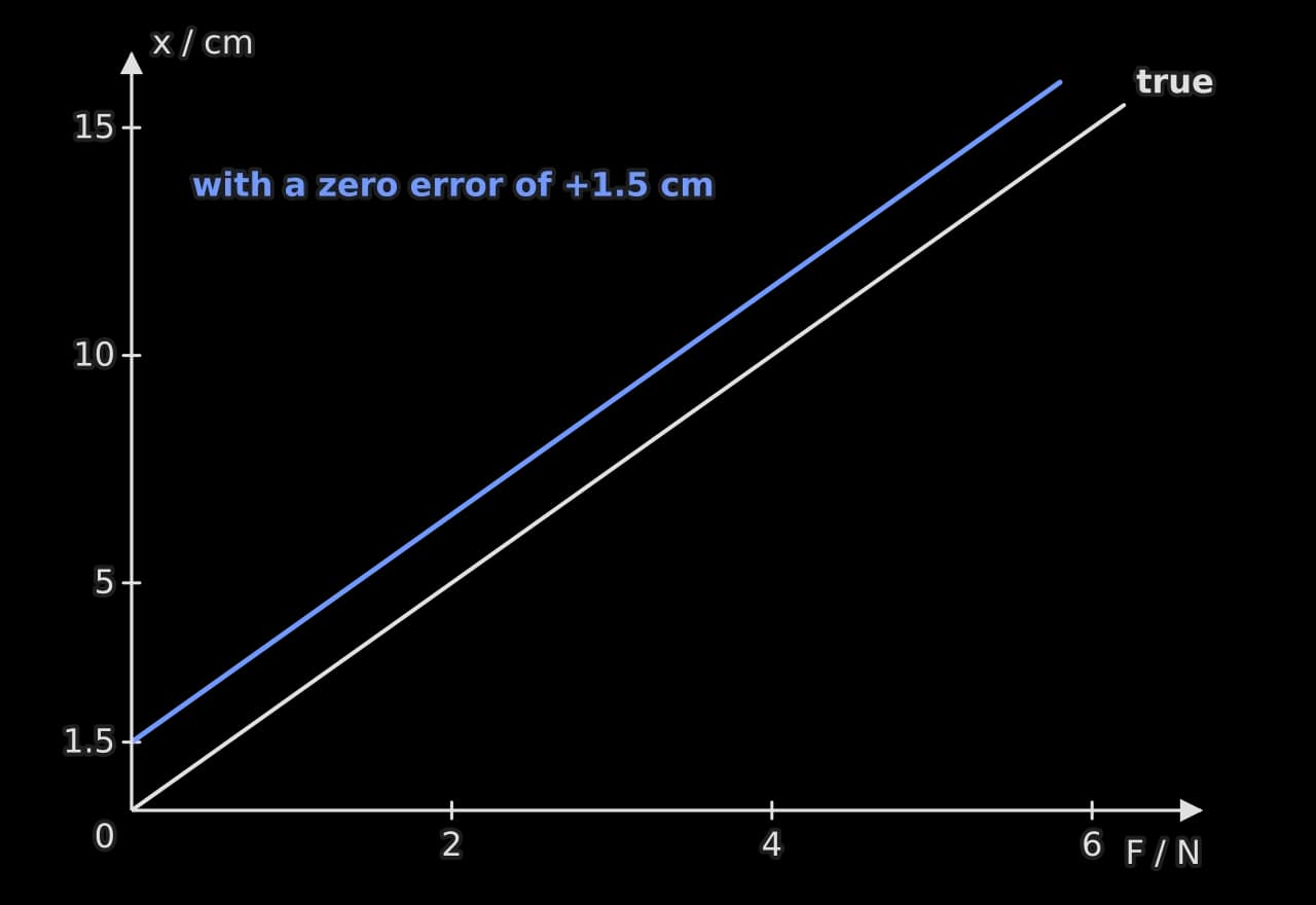
Graph of extension x in cm against force F in N. A black line passes through the origin, labelled true. A parallel blue line is shifted up to meet the vertical axis at 1.5 cm, labelled zero error of +1.5 cm. — A zero error adds the same amount to every reading, so the line moves up by that amount but keeps the same gradient.

This is why constants are usually found from gradients: a constant offset in all the readings of one variable moves the intercept but leaves the gradient unchanged. Correcting the zero error, by subtracting the zero reading from every value, removes the offset entirely.

Accuracy and precision

The two kinds of error correspond to two qualities of a set of measurements:

Precision is how closely repeated measurements agree with one another. Small random errors give high precision.
Accuracy is how close a measurement, or the mean of a set, is to the true value. Small systematic errors give high accuracy.

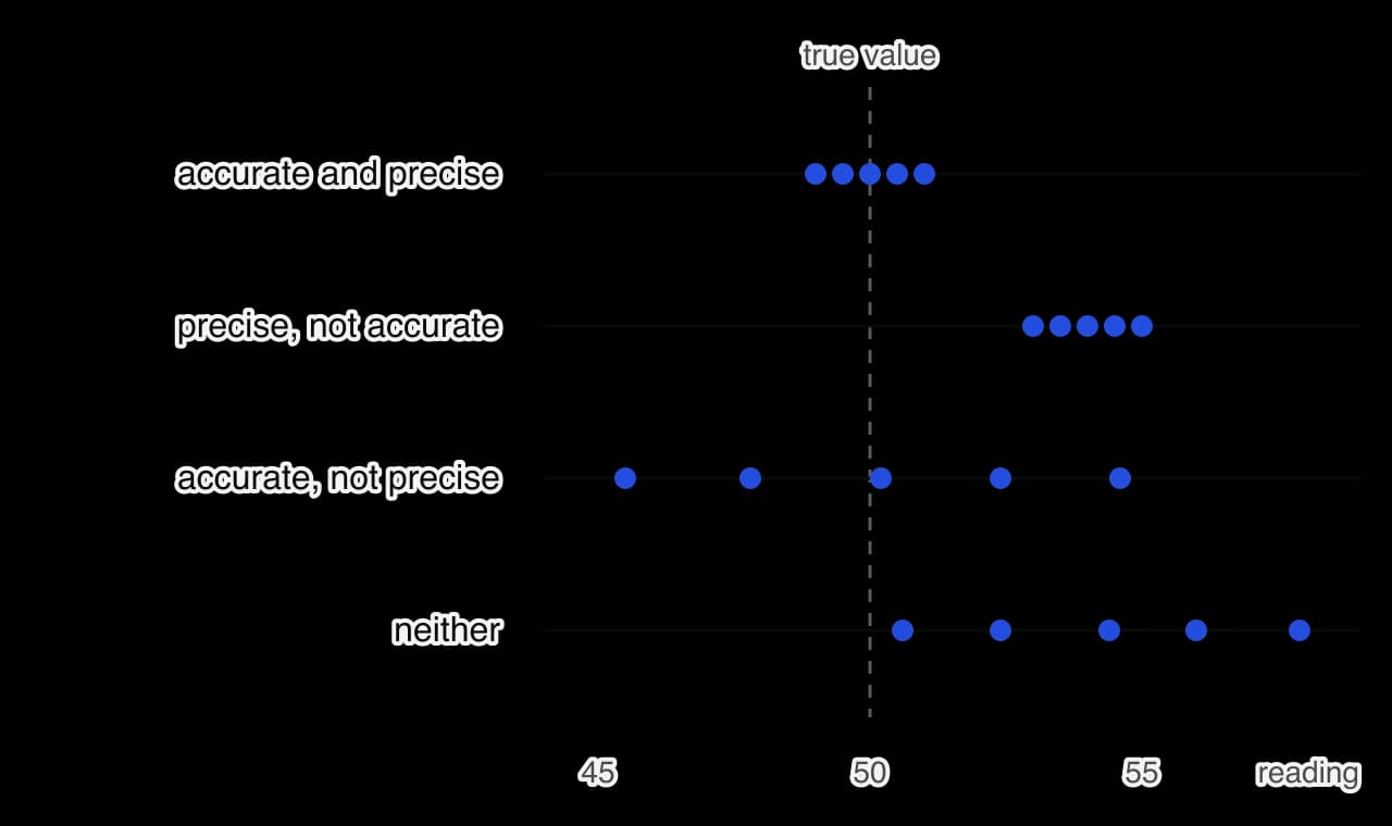
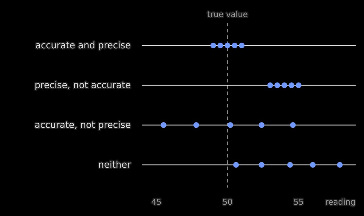
Four rows of five repeated readings, shown as blue dots on number lines, with a dashed vertical line at the true value of 50. Accurate and precise: dots clustered tightly round 50. Precise, not accurate: tight cluster round 54. Accurate, not precise: wide spread centred on 50. — Precision is how closely repeated readings agree with each other; accuracy is how close their mean is to the true value. Random errors spread the readings; a systematic error shifts them all.

A set of readings can be precise without being accurate (tightly grouped, but around the wrong value because of a systematic error), or accurate without being precise (widely scattered, but centred on the true value). Only a measurement with small random and small systematic errors is both.

Absolute, fractional and percentage uncertainty

An uncertainty can be expressed in three ways, each useful for a different calculation.

Measurement	Absolute	Fractional	Percentage
$(24.6 \pm 0.1)$ cm	0.1 cm	0.004	0.4 %
$(1.42 \pm 0.02)$ s	0.02 s	0.014	1.4 %
$(0.32 \pm 0.01)$ mm	0.01 mm	0.031	3 %
$(5.0 \pm 0.5)$ V	0.5 V	0.10	10 %

Fractional and percentage uncertainties have no unit, so they allow the precision of quantities with different units to be compared. The same absolute uncertainty is a much larger fraction of a small value than of a large one, which is why short lengths and short times are the least precise measurements in most experiments.

Writing an uncertainty

Give the absolute uncertainty to one significant figure (two are acceptable when the first digit is 1).
Round the value to the same decimal place as the uncertainty: $(9.86 \pm 0.24)$ becomes $(9.9 \pm 0.2)$ , and $(342.7 \pm 23)$ becomes $(340 \pm 20)$ .
Put the value and the uncertainty in brackets before the unit, or give the unit with both: $(2.66 \pm 0.06) {g cm}^{- 3}$ .

Estimating the uncertainty of a measurement

For a single reading, the uncertainty comes from the instrument and the way it is used: ± the last digit on a digital meter, ± half the smallest division on an analogue scale read at one point, and larger values where judgement is involved, such as human reaction time of about 0.1–0.2 s in hand timing. For repeated readings, the mean is the best value and half the range is a simple estimate of its uncertainty:

Δ x \approx \frac{x_{max} - x_{min}}{2}

When the scatter of repeated readings is larger than the instrument uncertainty, the scatter is the better estimate. When all repeats agree exactly, the instrument uncertainty is used instead.

Propagating uncertainties

When a result is calculated from measured quantities, its uncertainty is found from theirs. The data booklet gives three rules, which cover every calculation needed.

Operation	Rule
Addition or subtraction: $y = a \pm b$	$Δ y = Δ a + Δ b$
Multiplication or division: $y = \frac{a b}{c}$	$\frac{Δ y}{y} = \frac{Δ a}{a} + \frac{Δ b}{b} + \frac{Δ c}{c}$
Power: $y = a^{n}$	$\frac{Δ y}{y} = ∣ n \frac{Δ a}{a} ∣$

Each rule gives the largest likely uncertainty, assuming the individual errors combine in the worst way. Pure numbers and constants such as 2, π or $g$ from the data booklet have no uncertainty and do not contribute.

Sums and differences

For addition and subtraction the absolute uncertainties add, even when the quantities are subtracted. This makes a small difference between two large readings very uncertain.

Products and quotients

For multiplication and division the fractional (or percentage) uncertainties add. Convert each uncertainty to a fraction, add them, and multiply by the calculated value to return to an absolute uncertainty.

A rectangular metal block has mass $(54.2 \pm 0.1)$ g and sides $(3.00 \pm 0.02)$ cm, $(2.00 \pm 0.02)$ cm and $(3.40 \pm 0.02)$ cm. Determine its density with its absolute uncertainty.

Show the solution

\begin{aligned} V & = 3.00 \times 2.00 \times 3.40 = 20.4 {cm}^{3} \\ ρ & = \frac{m}{V} = \frac{54.2}{20.4} = 2.657 {g cm}^{- 3} \end{aligned}

Fractional uncertainties.

\begin{aligned} \frac{Δ ρ}{ρ} & = \frac{0.1}{54.2} + \frac{0.02}{3.00} + \frac{0.02}{2.00} + \frac{0.02}{3.40} \\ = 0.0018 + 0.0067 + 0.0100 + 0.0059 = 0.024 \\ Δ ρ & = 0.024 \times 2.657 = 0.06 {g cm}^{- 3} \end{aligned}

So $ρ = (2.66 \pm 0.06) {g cm}^{- 3}$ , or $(2.66 \pm 0.06) \times 10^{3} {kg m}^{- 3}$ . The shortest side contributes most, because the same 0.02 cm uncertainty is the largest fraction of it. The density of aluminium, $2.70 \times 10^{3} {kg m}^{- 3}$ , lies within the range, so the block could be aluminium.

Powers

A quantity raised to a power $n$ has its fractional uncertainty multiplied by $∣ n ∣$ . Squaring doubles the fractional uncertainty, cubing triples it, and a square root halves it ( $n = \frac{1}{2}$ ). Inverse quantities ( $n = - 1$ ) have the same fractional uncertainty as the original.

A student measures a pendulum of length $l = (0.800 \pm 0.002)$ m and finds its period to be $T = (1.79 \pm 0.02)$ s. Determine $g$ from $g = \frac{4 π^{2} l}{T^{2}}$ , with its uncertainty.

Show the solution

g = \frac{4 π^{2} \times 0.800}{{1.79}^{2}} = 9.857 {m s}^{- 2}

Fractional uncertainty. $4 π^{2}$ is exact. $l$ contributes once and $T$ twice, because it is squared:

\begin{aligned} \frac{Δ g}{g} & = \frac{Δ l}{l} + 2 \frac{Δ T}{T} = \frac{0.002}{0.800} + 2 \times \frac{0.02}{1.79} \\ = 0.0025 + 0.0223 = 0.0248 \\ Δ g & = 0.0248 \times 9.857 = 0.24 {m s}^{- 2} \end{aligned}

So $g = (9.9 \pm 0.2) {m s}^{- 2}$ . The accepted value, 9.8 m s⁻², lies within the range 9.7–10.1 m s⁻², so the result is consistent with it. Almost all of the uncertainty comes from the period: timing more oscillations would improve the result far more than measuring the length more precisely.

Percentage uncertainty and percentage error

Two different percentages describe the quality of a result. The percentage uncertainty comes from the experiment itself and says how precise the result is. The percentage error (or percentage difference) compares the result with an accepted value and says how accurate it is:

percentage error = \frac{∣ experimental value - accepted value ∣}{accepted value} \times 100 %

If the percentage error is smaller than the percentage uncertainty, the result agrees with the accepted value within its uncertainty, and random errors can explain the difference. If the percentage error is larger, a systematic error has probably affected the result, or the uncertainty has been underestimated.

Plotting a good graph

A graph used to analyse data follows a few conventions:

The independent variable goes on the horizontal axis and the dependent variable on the vertical axis.
Each axis is labelled with the quantity and its unit, separated by a slash: " $F$ / N", " $T^{2}$ / s²".
The scales are simple (1, 2 or 5 units per division, never 3) and use most of the grid. They need not start at zero.
Points are plotted as small crosses or dots, with error bars where the uncertainty is visible at the scale used.
A single smooth line or curve of best fit is drawn, never a dot-to-dot line joining the points.

Vertical bars show the uncertainty in the quantity on the vertical axis, and horizontal bars that on the horizontal axis. A point may have both, forming a cross. When the uncertainty in one quantity is too small to draw at the scale of the graph, its bars are left off, and it is good practice to say so.

Error bars for calculated quantities

When the plotted quantity is calculated from a measurement, such as $T^{2}$ or $\frac{1}{d^{2}}$ , its error bars come from the propagation rules. Each point usually has a different error bar, because the fractional uncertainty changes from point to point.

$d$ / m ± 0.005	$\frac{1}{d^{2}}$ / m⁻²	Fractional uncertainty	Error bar on $\frac{1}{d^{2}}$ / m⁻²
0.200	25.0	$2 \times \frac{0.005}{0.200} = 0.050$	± 1.3
0.300	11.1	$2 \times \frac{0.005}{0.300} = 0.033$	± 0.4
0.500	4.00	$2 \times \frac{0.005}{0.500} = 0.020$	± 0.08

For $\frac{1}{d^{2}}$ the power is $- 2$ , so the fractional uncertainty is twice that of $d$ . The shortest distance has both the largest value of $\frac{1}{d^{2}}$ and the largest fractional uncertainty, so its error bar is by far the longest. A line of best fit should be guided more by the points with short error bars.

Lines of best fit

A line of best fit shows the trend of the data while averaging out their scatter. For a straight line, draw it with a ruler so that the points are spread evenly above and below it along its whole length, and so that it passes through as many error bars as possible, ideally all of them. It does not have to pass through any particular point, including the origin or the first point.

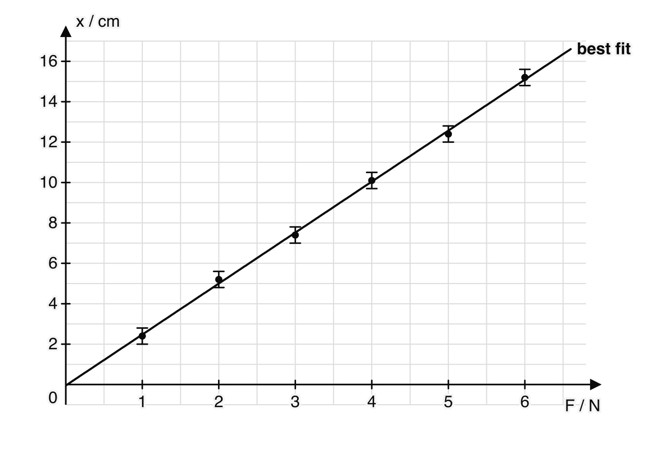
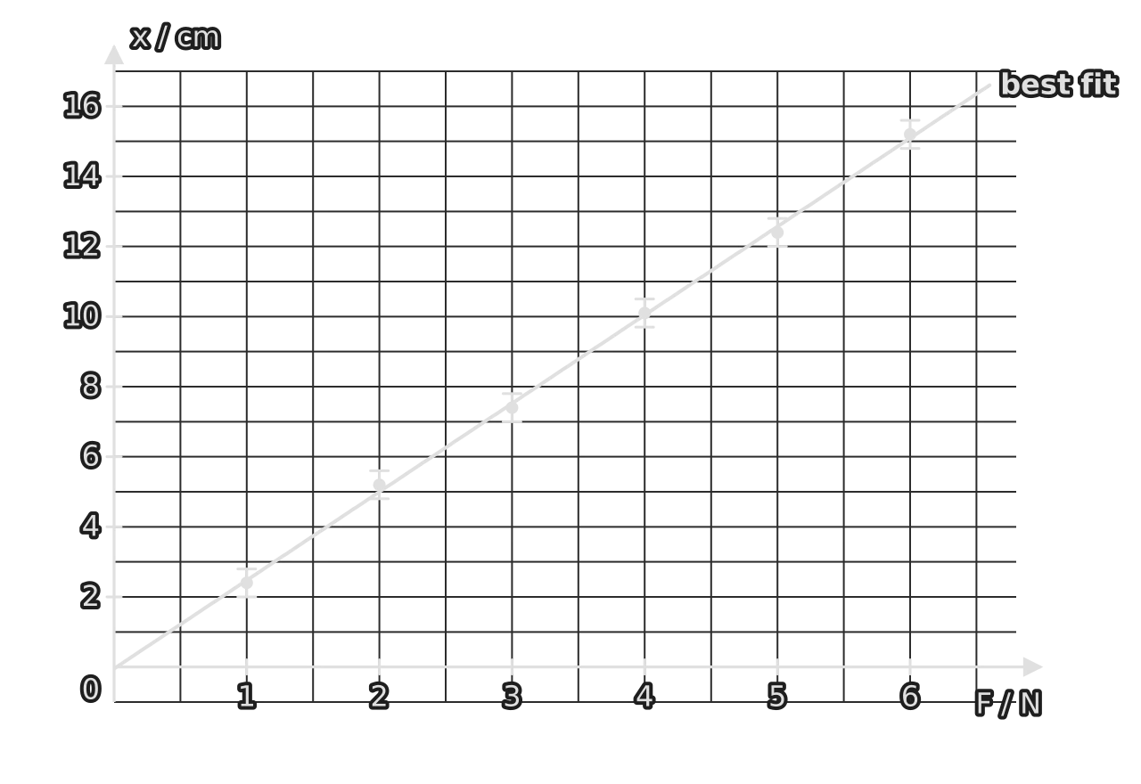
Graph of extension x in cm against load F in N, 1 to 6 N. Six points with vertical error bars of ±0.4 cm, from (1, 2.4) to (6, 15.2), lie on a straight best-fit line that passes through every error bar and through the origin. — A straight line passes through every error bar and through the origin, so the extension is directly proportional to the load. The line is not forced through any individual point.

The spring data show a straight line passing through every error bar and through the origin. The line is therefore consistent with direct proportionality between extension and load, which is Hooke’s law for this spring.

Linear or proportional?

The relationship is linear if a straight line can be drawn through all the error bars.
It is directly proportional if, in addition, that line passes through the origin (within the uncertainty of the intercept).

A point whose error bar is far from the line drawn through all the others is an outlier. It should be checked, and if a cause can be found or suspected (a misread scale, a miscounted oscillation), the measurement is repeated or the point is left out of the line and the omission stated.

Gradient and intercept

The gradient is found from a large triangle on the line, using two points on the line that are far apart, not data points from the table. Its unit is the unit of the vertical axis divided by that of the horizontal axis. Comparing the line with the theoretical equation gives the meaning of the gradient and intercept.

Uncertainty in the gradient and intercept

The gradient of the best-fit line is the best value, but other lines would also be consistent with the data. The uncertainty in the gradient is found from the steepest and the shallowest straight lines that still pass through every error bar, drawn by eye.

Draw the steepest line that still passes through every error bar. It usually runs from the bottom of the bars at the low end of the line to the top of the bars at the high end, but any bar in between can limit it.
Draw the shallowest line that passes through every error bar in the same way.
Find the gradient of each line from a large triangle.
Take the uncertainty in the gradient as half the difference between them, the usual method.

Δ m = \frac{m_{max} - m_{min}}{2}

The same spring data with the best-fit line in black, a steeper blue maximum-gradient line (gradient 2.67 cm per N, intercept −0.53 cm) and a shallower orange minimum-gradient line (gradient 2.40 cm per N, intercept +0.40 cm). Both pass through every error bar. — The steepest (blue) and shallowest (orange) straight lines that still pass through every error bar. Half the difference of their gradients is the uncertainty in the gradient; their intercepts give the uncertainty in the intercept.

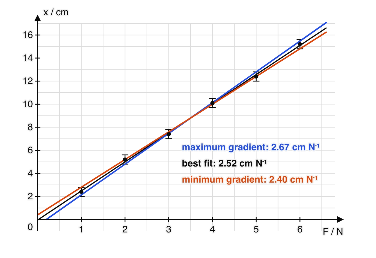
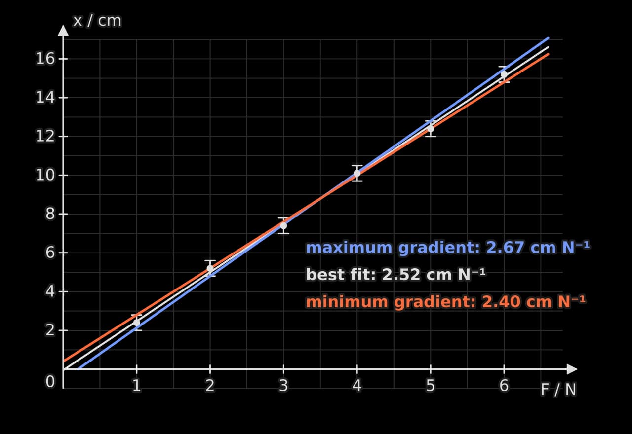
For the spring, the extreme lines have gradients 2.67 and 2.40 cm N⁻¹, so $Δ m = \frac{2.67 - 2.40}{2} \approx 0.13 {cm N}^{- 1}$ , an uncertainty of about 5 %. The maximum line is limited by the bars of the second and fifth points, not the first and last, which is why each line must be checked against every bar.

The same two lines give the uncertainty in the intercept. Their intercepts on the vertical axis are $- 0.53$ cm and $+ 0.40$ cm, so the intercept is about $(0.0 \pm 0.5)$ cm. Zero lies within this range, which confirms that the data are consistent with direct proportionality.

What the intercept shows

When theory predicts a line through the origin, the uncertainty range of the intercept is a test of the theory and of the method. If zero lies outside the range, there is a systematic error in one of the variables, and the size of the intercept measures it.

Linearising data

Many relationships in physics are curves. A curve is hard to test by eye: it is difficult to tell whether data follow $y \propto x^{2}$ or $y \propto x^{1.8}$ , and a constant cannot be read from it directly. The solution is to plot two quantities that the theory predicts are in a straight-line relation, a process called linearisation.

The pendulum is the standard example. The period is predicted to be $T = 2 π \sqrt{\frac{l}{g}}$ . A graph of $T$ against $l$ is a curve.

Graph of period T in s against length l in m for a pendulum. Five points from (0.2, 0.90) to (1.0, 2.01) lie on a smooth curve through the origin whose gradient decreases. — The period rises with length, but the curve flattens, so neither a straight line nor the value of g can be read from it directly.

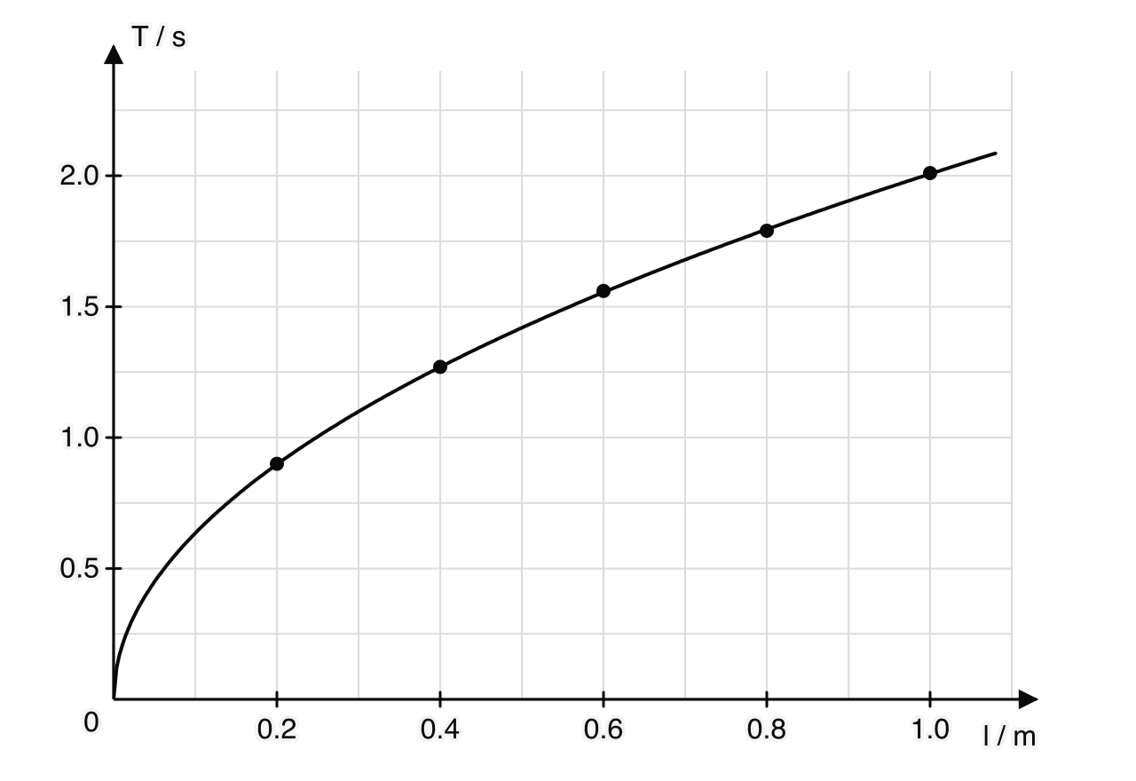
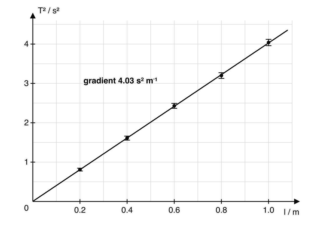
Squaring the equation gives $T^{2} = \frac{4 π^{2}}{g} l$ , which has the form $y = m x$ with $y = T^{2}$ , $x = l$ and gradient $m = \frac{4 π^{2}}{g}$ . A graph of $T^{2}$ against $l$ should therefore be a straight line through the origin. The error bars on $T^{2}$ are found with the power rule: a 1 % uncertainty in $T$ is a 2 % uncertainty in $T^{2}$ .

Graph of T squared in s² against length l in m. Five points with small vertical error bars, growing from ±0.04 to ±0.08 s², lie on a straight line through the origin with gradient 4.03 s² per m. — Plotting T² against l turns the curve into a straight line through the origin. Its gradient, 4π²/g, gives g.

The best-fit line of $T^{2}$ against $l$ has a gradient of 4.03 s² m⁻¹, and the maximum and minimum gradient lines have gradients 4.16 and 3.89 s² m⁻¹. Determine $g$ with its uncertainty.

Show the solution

g = \frac{4 π^{2}}{gradient} = \frac{4 π^{2}}{4.03} = 9.80 {m s}^{- 2}

Uncertainty. $Δ m = \frac{4.16 - 3.89}{2} = 0.135$ , a fractional uncertainty of $\frac{0.135}{4.03} = 0.034$ . Since $g \propto m^{- 1}$ , $g$ has the same fractional uncertainty: $Δ g = 0.034 \times 9.80 = 0.33 {m s}^{- 2}$ .

So $g = (9.8 \pm 0.3) {m s}^{- 2}$ , in agreement with the accepted value. Using five lengths and a gradient makes the result less sensitive to any one reading than the single-pendulum calculation, and an offset in the lengths (measuring to the top of the bob, say) would change only the intercept.

Common linearisations

Relationship	Plot $y$	against $x$	Gradient	Intercept
$y = k x^{2}$ (e.g. $s = \frac{1}{2} a t^{2}$ )	$s$	$t^{2}$	$\frac{1}{2} a$	0
$y = \frac{k}{x}$ (e.g. $p = \frac{n R T}{V}$ )	$p$	$\frac{1}{V}$	$n R T$	0
$y = \frac{k}{x^{2}}$ (e.g. $I = \frac{P}{4 π d^{2}}$ )	$I$	$\frac{1}{d^{2}}$	$\frac{P}{4 π}$	0
$y = a + b x^{2}$	$y$	$x^{2}$	$b$	$a$
$y = k x^{n}$ , $n$ unknown	$\lg y$	$\lg x$	$n$	$\lg k$
$y = y_{0} e^{- k x}$ (e.g. $N = N_{0} e^{- λ t}$ )	$\ln y$	$x$	$- k$	$\ln y_{0}$

Logarithmic graphs

Finding an unknown power

When a relationship is thought to be a power law, $y = k x^{n}$ , but the power $n$ is unknown, taking logarithms of both sides gives a straight line:

\lg y = n \lg x + \lg k

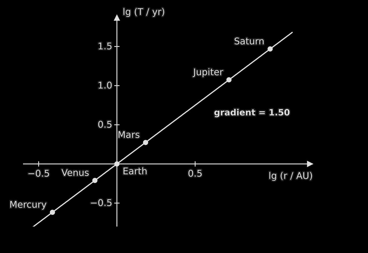
A graph of $\lg y$ against $\lg x$ (a log–log graph) is then a straight line with gradient $n$ and intercept $\lg k$ . Logarithms to base 10 (lg) or base e (ln) both work, as long as the same base is used for both axes. Logarithms have no units, so the quantities are divided by their units before the logarithm is taken: the axis is labelled "lg (r / AU)", not "lg r / AU".

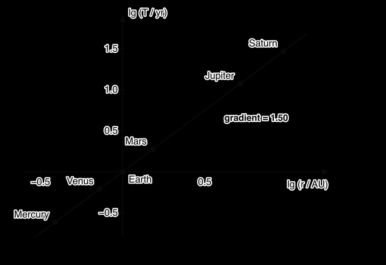
The orbits of the planets give a real example. Plotting the logarithm of each planet’s orbital period against the logarithm of its orbital radius, both relative to the Earth’s, gives a straight line.

Graph of lg of orbital period (in years) against lg of orbital radius (in AU) for six planets from Mercury to Saturn. The points lie on a straight line through the origin, at Earth, with gradient 1.50. — A log–log graph of the planets’ orbits is a straight line of gradient 1.50, so T ∝ r^1.5, which is Kepler’s third law. Data: semi-major axes from NASA JPL approximate planetary orbital elements (epoch J2000); sidereal periods from the NASA Planetary Fact Sheet (accessed 2026).

Exponential relationships

An exponential relationship such as radioactive decay, $N = N_{0} e^{- λ t}$ , becomes straight when the natural logarithm of $N$ is plotted against $t$ : $\ln N = - λ t + \ln N_{0}$ . The gradient is $- λ$ and the intercept is $\ln N_{0}$ . Any quantity proportional to $N$ , such as the activity or the corrected count rate, gives the same gradient.

Logarithmic scales

A logarithmic scale is an axis on which equal distances represent equal factors, usually factors of ten, rather than equal steps. It is used when data span many orders of magnitude, so that very small and very large values can be shown together: the luminosity axis of the Hertzsprung–Russell diagram, the electromagnetic spectrum and the sound intensity scale are examples. Reading such a scale means remembering that the point halfway between $10^{2}$ and $10^{3}$ is about 316, not 550.

Reducing uncertainties in practice

The analysis of uncertainties points directly at the most useful improvements to an experiment. The largest fractional uncertainty, after multiplying by its power, limits the result; reducing a small contribution further changes almost nothing. Each kind of improvement acts on a particular kind of error.

Technique	What it reduces	Example
Repeat readings and take the mean	Random error	Time the fall of a ball five times
Measure a multiple of the quantity	Fractional uncertainty from resolution or reaction time	Time 20 oscillations; measure the thickness of 100 sheets of paper
Increase the size of the quantity measured	Fractional uncertainty	Heat the water through a larger temperature rise; use a longer wire
Use an instrument with finer resolution	Uncertainty of each reading	Micrometer instead of a rule for a wire diameter
Widen the range and add more points	Uncertainty in the gradient	Five lengths from 0.20 m to 1.00 m instead of three from 0.40 m to 0.60 m
Correct a zero error; calibrate the instrument	Systematic error	Subtract the reading with no load; check a thermometer in ice and boiling water
Change the method to remove a loss	Systematic error	Insulate a calorimeter; use a light gate instead of hand timing

An improvement is only worth suggesting if it acts on the uncertainty that dominates. In the pendulum calculation of $g$ , the period contributed 2.2 % and the length 0.25 %; timing twice as many oscillations would almost halve the uncertainty in $g$ , while a better metre rule would make no visible difference.

Reading a graph

Once a graph is drawn, its features carry physical meaning:

The gradient is the rate of change of the vertical quantity with the horizontal one: velocity on a displacement–time graph, acceleration on a velocity–time graph, resistance on a straight $V$ – $I$ graph through the origin.
The area under the line is the product of the two quantities: displacement under a velocity–time graph, impulse under a force–time graph, work done under a force–extension graph.
An intercept is the value of one quantity when the other is zero: the emf on a $V$ – $I$ graph of a cell, absolute zero, found by extrapolating a graph of gas pressure against temperature in °C to zero pressure.
A change of gradient, a maximum or a minimum marks where the behaviour changes, such as the limit of proportionality of a spring or the resonant frequency of an oscillator.
Interpolation reads values between the measured points; extrapolation extends the line beyond them and is less reliable, because the relationship may change outside the measured range.

Self-check

To do:
I can distinguish random and systematic errors, give examples of each and say how each is reduced.
To do:
I can explain the difference between accuracy and precision.
To do:
I can express an uncertainty as absolute, fractional and percentage, and quote a value and its uncertainty to consistent precision.
To do:
I can estimate the uncertainty of a single reading and of a set of repeated readings.
To do:
I can propagate uncertainties through sums, differences, products, quotients and powers.
To do:
I can compare a result with an accepted value using its percentage uncertainty and percentage error.
To do:
I can plot a graph with labelled axes, sensible scales and error bars, and draw a line of best fit.
To do:
I can decide whether data are linear or directly proportional.
To do:
I can find a gradient and an intercept with units, and their uncertainties from maximum and minimum gradient lines.
To do:
I can linearise a relationship and find a constant from the gradient or intercept.
To do:
I can use a log–log graph to find an unknown power, and a log–linear graph for an exponential relationship.

Carry on with Physics in Augment

With a free account, Augment remembers where you stopped in the notes and which questions you have marked.

Start free