Paper 1B: data-based questions

What Paper 1B tests and how to answer it: reading experimental data, uncertainties, graphs with error bars, gradients and intercepts, linearising, and evaluating an experiment, with fully worked examples.

IB Physics
Exam skills
SL and HL

18 min readLast reviewed 14 Oct 2026

Paper 1B is the data-based part of Paper 1. Its questions describe an experiment of the kind carried out in a school laboratory, usually by "a group of students", and then work through the skills of handling real data: the uncertainty in a reading, the processing of repeated measurements, a graph with error bars, a gradient and its unit, the meaning of an intercept, and a judgement about how good the result is. The same questions are set at SL and HL.

The physics in a Paper 1B question may be unfamiliar. When it is, every relationship needed is given in the stem, and the marks are for using it, not for knowing it in advance. The question is testing whether you can think like an experimenter.

Reading the experiment and its data

Start by reading the whole stem and identifying the variables. The independent variable is the one the students change deliberately; the dependent variable is the one they measure as a result; control variables are kept constant so that they do not affect the result. Then read the data table carefully, because its headings carry information.

A column heading in IB style gives the quantity, its unit and its uncertainty: " $d$ / cm ± 0.1" means every value in the column is a distance in centimetres with an absolute uncertainty of 0.1 cm. All values in a column should have the same number of decimal places, matching the uncertainty. A value written as 12.0 cm was read to the nearest millimetre; one written as 12 cm was not.

$m$ / kg ± 0.001	$t_{1}$ / s ± 0.01	$t_{2}$ / s ± 0.01	$t_{3}$ / s ± 0.01	mean $t$ / s
0.050	1.42	1.39	1.45	1.42
0.100	1.03	1.08	1.01	1.04
0.150	0.86	0.84	0.89	0.86

This table shows the standard layout: the independent variable in the first column, repeated trials of the dependent variable, and a processed column (the mean). Each mean is given to the same decimal places as the raw data.

Uncertainty in a single reading

Every reading has an uncertainty. For a single reading the usual conventions are:

Digital instruments: ± the smallest digit shown (a balance reading 24.37 g is ± 0.01 g).
Analogue scales: ± half the smallest division, if the reading can be made at a single point (a thermometer with 1 °C divisions is ± 0.5 °C).
Lengths measured with a rule: often ± 1 mm, because two ends are read, each to ± 0.5 mm.
Human timing: the reaction time, about ± 0.1 to 0.2 s, is much larger than the stopwatch resolution of 0.01 s.

The last point leads to a technique Paper 1B often asks about. When the uncertainty in starting and stopping a stopwatch is about 0.2 s, timing one swing of a pendulum with a period of about 1.4 s gives an uncertainty of about 14 %. Timing 20 swings in one go keeps the same absolute uncertainty in the total time, but the period is the total divided by 20, so its uncertainty is $\frac{0.2}{20} = 0.01 s$ .

Repeated readings and outliers

When a measurement is repeated, the best value is the mean of the readings. A simple estimate of its uncertainty, accepted in IB markschemes, is half the range:

Δ x = \frac{x_{max} - x_{min}}{2}

If the readings all agree exactly, the uncertainty is the instrument uncertainty instead. Repeating readings reduces the effect of random errors (the scatter), but it does not reduce a systematic error, which shifts every reading by the same amount.

An outlier is a reading that lies far from the others for a reason that can be identified or suspected, such as a misread scale or a miscounted oscillation. It is excluded from the mean, and the exclusion is stated. No calculation is needed to identify an outlier; it is a judgement based on the spread of the other readings.

Uncertainties in processed data

Paper 1B often asks for the uncertainty in a quantity calculated from the readings. The rules in the data booklet cover every case:

Calculation	Rule	Example
Sum or difference: $y = a \pm b$	Add absolute uncertainties: $Δ y = Δ a + Δ b$	Two lengths of $(12.0 \pm 0.1)$ cm and $(4.5 \pm 0.1)$ cm: difference $(7.5 \pm 0.2)$ cm
Product or quotient: $y = \frac{a b}{c}$	Add fractional uncertainties: $\frac{Δ y}{y} = \frac{Δ a}{a} + \frac{Δ b}{b} + \frac{Δ c}{c}$	$R = \frac{V}{I}$ with 2 % in $V$ and 3 % in $I$ : 5 % in $R$
Power: $y = a^{n}$	Multiply the fractional uncertainty by $∣ n ∣$ : $\frac{Δ y}{y} = ∣ n \frac{Δ a}{a} ∣$	$T^{2}$ with 1 % in $T$ : 2 % in $T^{2}$

The method is always the same: convert to fractional (or percentage) uncertainties for products, quotients and powers, combine them, then convert back to an absolute uncertainty by multiplying by the value.

The largest fractional uncertainty

When every reading in a column has the same absolute uncertainty, the fractional uncertainty is largest for the smallest reading. A length of $(2.0 \pm 0.1)$ cm has a 5 % uncertainty, while $(20.0 \pm 0.1)$ cm has only 0.5 %. Questions that ask for "the largest percentage uncertainty in the data" expect you to choose the smallest value, not to calculate every one.

The diameter of a wire is measured with a micrometer as $(0.32 \pm 0.01)$ mm and its length as $(80.0 \pm 0.2)$ cm. Its resistance is $(5.4 \pm 0.1) Ω$ . The resistivity is $ρ = \frac{R A}{L}$ with $A = \frac{π d^{2}}{4}$ . Calculate the percentage uncertainty in $ρ$ .

Show the solution

Fractional uncertainty in each quantity.

\begin{aligned} \frac{Δ R}{R} & = \frac{0.1}{5.4} = 1.9 % \\ \frac{Δ d}{d} & = \frac{0.01}{0.32} = 3.1 % \Rightarrow \frac{Δ A}{A} = 2 \times 3.1 = 6.3 % \\ \frac{Δ L}{L} & = \frac{0.2}{80.0} = 0.25 % \end{aligned}

Combine. $ρ$ is a product and quotient, so the percentages add: $1.9 + 6.3 + 0.25 = 8.4 % \approx 8 %$ .

The diameter contributes most, because it is the smallest measurement and it is squared. A better result would come from measuring the diameter at several points along the wire and averaging, since the micrometer cannot be read more finely.

Graphs with error bars

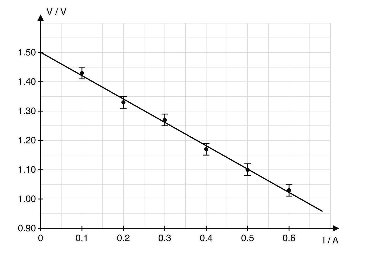
A Paper 1B graph is usually already drawn, with error bars on the points. An error bar extends from the plotted value by the absolute uncertainty in each direction, so its total length is twice the uncertainty. Bars may be vertical (uncertainty in the dependent variable), horizontal (independent variable), or both. When the uncertainty in one variable is too small to show at the scale of the graph, its bars are left off, and a question may ask why.

Linear or proportional?

Two words describe a straight-line relationship, and Paper 1B tests the difference:

Linear: a single straight line can be drawn through all the error bars.
Directly proportional: the relationship is linear and the line also passes through the origin (within the uncertainties).

A line that misses one error bar is not enough to reject a linear relationship if the bar is close; a line that cannot pass through several of them shows the relationship is not linear. When asked "Outline why the graph is not linear", refer to the error bars: "no straight line can be drawn through all the error bars".

Gradients and intercepts

To find a gradient, draw a large triangle on the best-fit line, using at least half of the line, and read two points that lie on the line itself, not data points. The gradient has a unit: the unit of the vertical axis divided by that of the horizontal one. Its physical meaning comes from comparing the equation of the straight line, $y = m x + c$ , with the theoretical equation.

The intercept is the value of $y$ when $x = 0$ . If the horizontal axis does not start at zero, the intercept cannot be read directly from where the line meets the vertical axis; extend the line, or calculate $c = y - m x$ from a point on the line.

Graph of terminal pd V in volts (axis from 0.90 to 1.60 V) against current I in amperes from 0 to 0.7 A. Six points with error bars of ±0.02 V fall on a straight line sloping down from 1.50 V at I = 0 to about 1.02 V at 0.6 A. — The variation of terminal pd V with current I for a cell. The vertical axis starts at 0.90 V, so the intercept on the V axis is read at I = 0.

The terminal pd $V$ of a cell is measured for different currents $I$ , giving the graph of $V$ against $I$ . The cell obeys $V = ε - I r$ . The maximum and minimum gradient lines through the error bars have gradients $- 0.85 Ω$ and $- 0.73 Ω$ . Determine the emf $ε$ and the internal resistance $r$ with its uncertainty.

Show the solution

Match the equation. $V = - r I + ε$ has the form $y = m x + c$ with gradient $- r$ and intercept $ε$ .

Intercept. The best-fit line meets $I = 0$ at $V = 1.50 V$ , so $ε = 1.50 V$ .

Gradient. From two points on the line, $(0.00, 1.50)$ and $(0.60, 1.02)$ :

m = \frac{1.02 - 1.50}{0.60 - 0.00} = - 0.80 Ω \Rightarrow r = 0.80 Ω

Uncertainty. Half the difference of the extreme gradients: $Δ r = \frac{0.85 - 0.73}{2} = 0.06 Ω$ . So $r = (0.80 \pm 0.06) Ω$ .

A gradient of V / A has the unit of resistance, the ohm, as expected for an internal resistance.

Linearising to test a relationship

Many relationships in physics are not straight lines. A curve is hard to test by eye and hard to extract a constant from, so the data are plotted in a form that the theory predicts is a straight line. This is called linearisation. The method is to rearrange the equation into the form $y = m x + c$ , where $y$ and $x$ are quantities that can be calculated from the data and $m$ and $c$ contain the constants.

Relationship	Plot	Gradient	Intercept
$T = 2 π \sqrt{\frac{l}{g}}$	$T^{2}$ against $l$	$\frac{4 π^{2}}{g}$	0
$f = \frac{1}{2 L} \sqrt{\frac{F}{μ}}$	$f^{2}$ against $F$	$\frac{1}{4 L^{2} μ}$	0
$I = \frac{P}{4 π d^{2}}$	$I$ against $\frac{1}{d^{2}}$	$\frac{P}{4 π}$	0
$V = ε - I r$	$V$ against $I$	$- r$	$ε$
$T = a + b v^{2}$	$T$ against $v^{2}$	$b$	$a$
$y = k x^{n}$ ( $n$ unknown)	$\log y$ against $\log x$	$n$	$\log k$

The last row is the general method when the power is not known: taking logarithms of both sides turns any power law into a straight line whose gradient is the power. Paper 1B more often gives the relationship and asks why a particular graph was plotted.

Units of a constant from a gradient or an equation

A constant found from a graph has the unit of the gradient, which can be simplified into SI base units. Paper 1B also asks for the powers in an unfamiliar relationship, found by making the units of both sides agree.

The frequency $f$ of oscillation of a small liquid drop is thought to depend on the surface tension $γ$ of the liquid (unit ${N m}^{- 1}$ ), its density $ρ$ and the radius $r$ of the drop, as $f = k γ^{x} ρ^{y} r^{z}$ , where $k$ is a dimensionless constant. Determine $x$ , $y$ and $z$ .

Show the solution

Write every unit in SI base units. $f$ : $s^{- 1}$ . $γ$ : ${N m}^{- 1} = {kg s}^{- 2}$ . $ρ$ : ${kg m}^{- 3}$ . $r$ : m.

s^{- 1} = ({kg s}^{- 2})^{x} ({kg m}^{- 3})^{y} m^{z}

Match the powers of each base unit.

\begin{aligned} s: - 1 & = - 2 x & \Rightarrow x = \frac{1}{2} \\ kg: 0 & = x + y & \Rightarrow y = - \frac{1}{2} \\ m: 0 & = - 3 y + z & \Rightarrow z = - \frac{3}{2} \end{aligned}

So $f = k \sqrt{\frac{γ}{ρ r^{3}}}$ . Larger drops oscillate more slowly and stronger surface tension makes them oscillate faster, which is physically reasonable.

Systematic errors and what an intercept shows

When the theory predicts a line through the origin but the best-fit line misses it, the usual cause is a systematic error: every reading of one variable is shifted by the same amount. Typical sources are a zero error (a meter or balance that does not read zero when it should), a length measured to the wrong point, or a constant delay in a timing circuit.

A pendulum gives a clear example. The period depends on the length from the pivot to the centre of mass of the bob. If students measure only the string, from the pivot to the top of the bob, every length is too short by the radius $r$ of the bob. Then $T^{2} = \frac{4 π^{2}}{g} (l + r)$ , the line of $T^{2}$ against $l$ has a positive intercept on the $T^{2}$ axis, and it crosses the $l$ axis at $l = - r$ . The gradient is unchanged, so the value of $g$ from the gradient is still correct. This is one advantage of finding a constant from a gradient: a constant offset in one variable affects only the intercept.

Evaluating and improving an experiment

Comparing with an accepted value

A result is consistent with an accepted value if the accepted value lies within the experimental range, value ± uncertainty. A measured $g = (9.6 \pm 0.3) {m s}^{- 2}$ covers 9.3 to 9.9 m s⁻² and so agrees with 9.8 m s⁻². If the accepted value lies outside the range, there is probably a systematic error, or the uncertainty has been underestimated. The percentage error (or percentage difference) compares the two:

percentage error = \frac{∣ experimental - accepted ∣}{accepted} \times 100 %

Suggesting improvements

Suggestions must be specific and realistic for the apparatus described, and each needs a reason that links it to an uncertainty or an error. Markschemes accept improvements such as these:

Time many oscillations or many fringes, so the fractional uncertainty from reaction time or resolution is smaller.
Extend the range of the independent variable, or take more data points within it, so the gradient is better defined.
Repeat readings and average, to reduce random error.
Use an instrument with a finer resolution where it makes a difference: a micrometer instead of a rule for a wire diameter, a vernier caliper for a bob diameter.
Use a fiducial marker, a light gate or video analysis to judge a position or time more precisely.
Check and correct for a zero error before taking readings.

A complete Paper 1B question

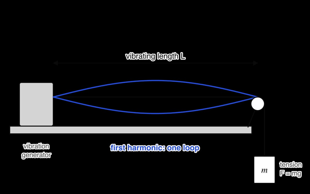
This question combines the skills of a whole Paper 1B question. A group of students investigates the first harmonic of a stretched string. The string runs from a vibration generator over a pulley to a hanging mass, which sets the tension $F$ . The vibrating length is $L = (0.800 \pm 0.002) m$ . For each tension the students adjust the frequency until the string vibrates in one loop, and record that frequency $f$ . Theory predicts $f = \frac{1}{2 L} \sqrt{\frac{F}{μ}}$ , where $μ$ is the mass per unit length of the string.

A string runs horizontally from a vibration generator on the left over a pulley on the right, where a hanging mass m pulls it taut with tension F = mg. The vibrating length L runs from the generator to the pulley. The string vibrates in one loop, drawn in blue. — The hanging mass sets the tension; the generator frequency is adjusted until the string vibrates in one large loop (the first harmonic).

The students’ results are:

$F$ / N ± 0.1	$f$ / Hz ± 1	$f^{2}$ / Hz²	$Δ (f^{2})$ / Hz²
2.0	28	784	?
4.0	40	1600	80
6.0	48	2304	96
8.0	55	3025	110
10.0	62	3844	124

Graph of f squared in Hz squared against tension F in newtons, from 2 to 10 N. Five points with vertical error bars growing from ±56 to ±124 Hz² lie close to a straight best-fit line passing near the origin and through about (10, 3820). — The variation of f² with F. The best-fit line passes through every error bar and very close to the origin, as f² ∝ F predicts.

(a) The signal generator displays the frequency to 0.1 Hz. Outline why the students recorded an uncertainty of ± 1 Hz. [1]

(b) Calculate the missing value of $Δ (f^{2})$ for $F = 2.0 N$ . [2]

(d) Determine, using the graph, the mass per unit length $μ$ of the string. [3]

(e) State the unit of the gradient of the graph in fundamental SI units. [1]

(f) The maximum and minimum gradient lines through the error bars have gradients of 401 Hz² N⁻¹ and 360 Hz² N⁻¹. Determine the absolute uncertainty in $μ$ . [2]

(g) The manufacturer states that $μ = 1.0 \times 10^{- 3} {kg m}^{- 1}$ . Comment on the students’ result. [1]

Show the markscheme

(a) the string vibrates with a large amplitude over a range of frequencies / judging the frequency of maximum amplitude by eye is imprecise ✓ OWTTE

(b) $\frac{Δ (f^{2})}{f^{2}} = 2 \times \frac{1}{28}$ « $= 0.071$ » ✓

$Δ (f^{2}) = 0.071 \times 784 = 56$ «Hz²» ✓

Award [2] for a bald correct answer. Accept 60 Hz².

(c) «squaring the equation gives» $f^{2} = \frac{1}{4 L^{2} μ} F$ / $f^{2} \propto F$ ✓

so the graph is a straight line through the origin with gradient $\frac{1}{4 L^{2} μ}$ «from which $μ$ can be found» ✓

(d) gradient from a large triangle on the line, eg $\frac{3820 - 50}{10.0 - 0}$ = 377 «Hz² N⁻¹» ✓

$μ = \frac{1}{4 L^{2} \times gradient} = \frac{1}{4 \times {0.800}^{2} \times 377}$ ✓

$μ = 1.04 \times 10^{- 3}$ «kg m⁻¹» ✓

Accept gradients in the range 365–390 Hz² N⁻¹ and answers in the range 1.00–1.07 × 10⁻³ kg m⁻¹. Allow ECF from an incorrect gradient for MP3.

(e) ${kg}^{- 1} m^{- 1}$ ✓

Hz² N⁻¹ = s⁻² ÷ kg m s⁻²; do not accept Hz² N⁻¹.

(f) fractional uncertainty in gradient $= \frac{(401 - 360) / 2}{377} = 5.4 %$ ✓

adding $2 \times \frac{0.002}{0.800} = 0.5 %$ for $L^{2}$ gives about 6 %, so $Δ μ = 0.06 \times 1.04 \times 10^{- 3} \approx 0.06 \times 10^{- 3}$ «kg m⁻¹» ✓

Allow 0.05 × 10⁻³ to 0.07 × 10⁻³ kg m⁻¹. Accept an answer that ignores the uncertainty in L, if it is stated to be negligible.

(g) the manufacturer’s value lies within the range $(1.04 \pm 0.06) \times 10^{- 3}$ « $0.98$ to $1.10 \times 10^{- 3}$ kg m⁻¹» so the result is consistent with it ✓

Allow ECF from (d) and (f).

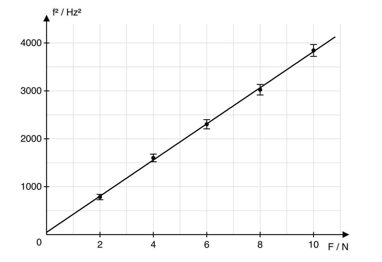
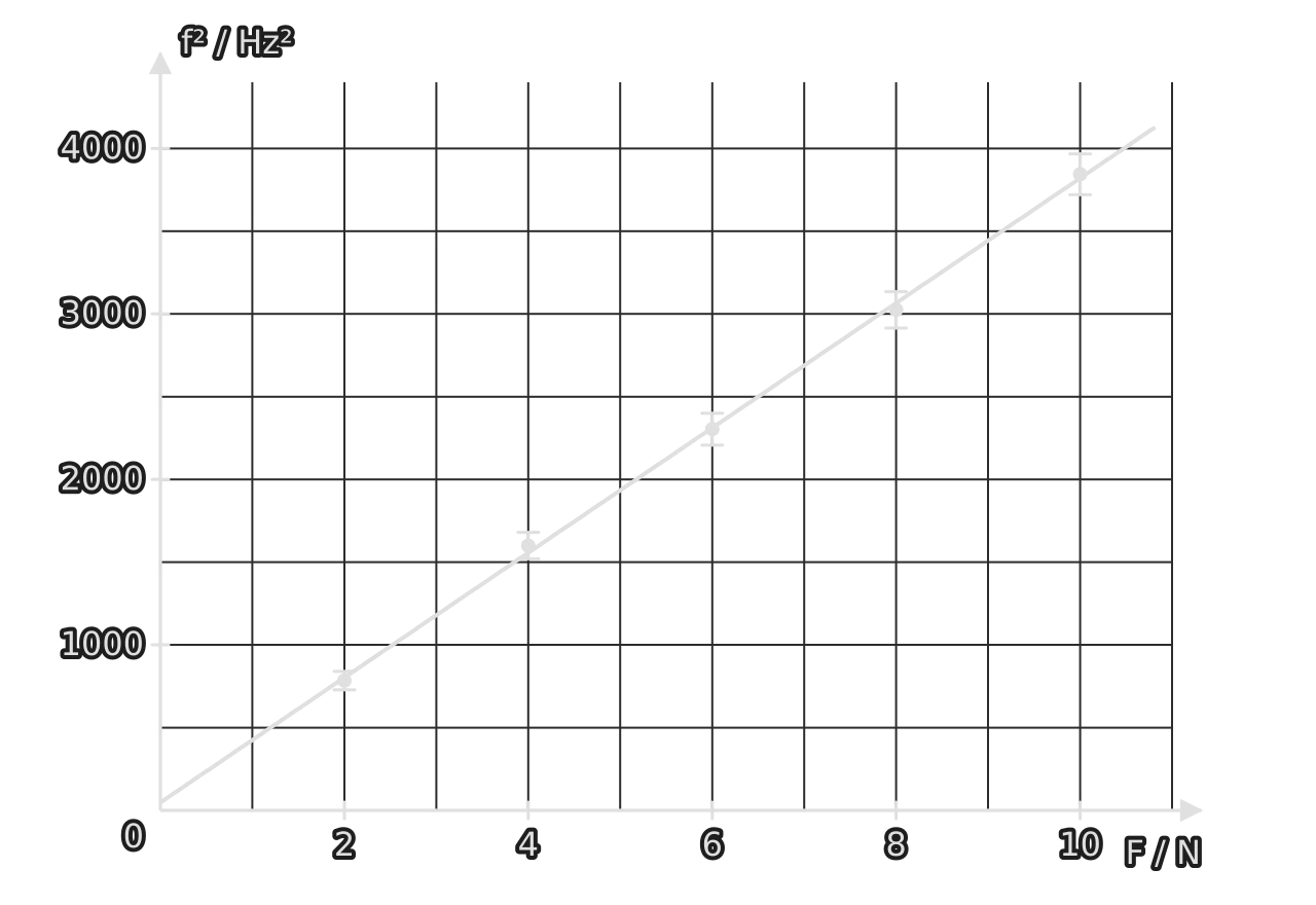
Part (f) shows the usual way to combine the uncertainty of a gradient with that of another measured quantity: find the fractional uncertainty of the gradient from the extreme lines, add the fractional uncertainties of everything else in the expression, and only then convert back to an absolute value.

Self-check

To do:
I can identify the independent, dependent and control variables in a described experiment.
To do:
I can read a table heading of the form "quantity / unit ± uncertainty" and write values to consistent decimal places.
To do:
I can state the uncertainty of a digital or analogue reading and of a hand-timed interval.
To do:
I can explain how timing many oscillations reduces the uncertainty in a period.
To do:
I can find the mean of repeated readings, its uncertainty as half the range, and justify leaving out an outlier.
To do:
I can propagate uncertainties through sums, products, quotients and powers, and find the largest fractional uncertainty in a data set.
To do:
I can decide whether a graph with error bars shows a linear or a proportional relationship.
To do:
I can find a gradient and an intercept with their units and physical meaning, and their uncertainties from extreme lines.
To do:
I can explain why a particular graph is plotted to linearise a relationship.
To do:
I can find the powers in an unfamiliar relationship from SI base units.
To do:
I can explain how a systematic error affects the intercept but not the gradient.
To do:
I can compare a result with an accepted value and suggest realistic improvements with reasons.

Carry on with Physics in Augment

With a free account, Augment remembers where you stopped in the notes and which questions you have marked.

Start free