Collecting, processing and presenting data
Choose and justify a sampling strategy, collect reliable primary data in rivers, on beaches and in towns, process it into tables, present it with the most appropriate graphs and maps, and apply Spearman’s rank and chi-squared tests.
- IB Geography
- Internal assessment
- SL and HL
Sampling
No investigation can measure everything: every metre of a river, every person in a town, every pebble on a beach. Sampling selects a manageable number of sites, people or items so that conclusions about the whole can be drawn from them. A good sample is large enough to show a pattern, spread across the whole study area, and chosen in a way that does not favour particular results.
Four sampling methods are used in geographical fieldwork. Each can be applied to points (sites in an area), lines (sites along a transect) or areas (squares of a grid), and to people as well as places.
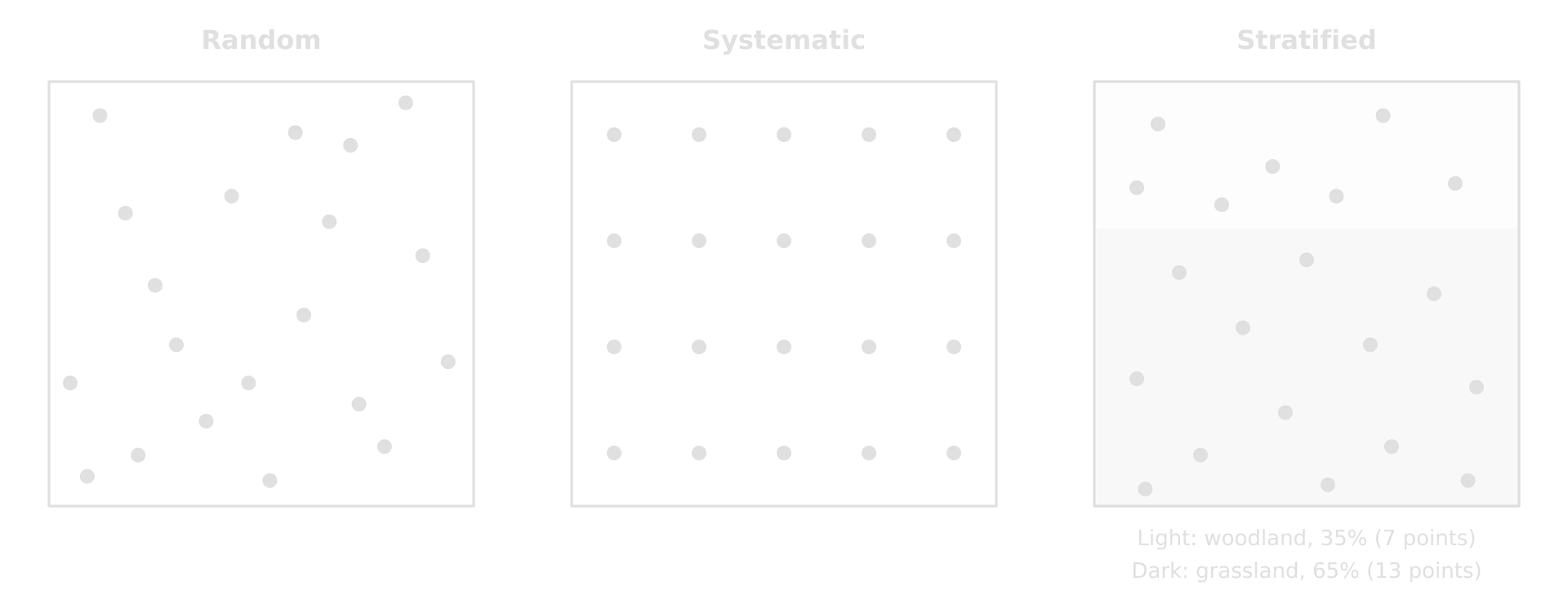
Method | How it works | Strengths | Limitations |
|---|---|---|---|
Every point or person has an equal chance of selection, chosen with random number tables or a random number generator (for example, grid coordinates) | Free from the investigator’s bias; suits statistical tests | May miss parts of the area by chance; random points may be inaccessible | |
Samples at regular intervals: every 50 m along a transect, every tenth passer-by, every 15 minutes | Easy to organise; even coverage; good for showing change with distance | May miss or over-represent features that recur at the same interval | |
The population or area is divided into subgroups (land-use zones, age groups) and each is sampled in proportion to its share | Every subgroup is represented in the right proportion | Needs reliable information on the size of each subgroup | |
Pragmatic sampling (opportunistic) | Sites or people are chosen because they are safe, accessible and available | Practical where access is limited; often the only safe option on a river | Most open to bias; results may not represent the whole |
Methods are often combined. A transect may use systematic sites, adjusted pragmatically where a site falls in a private garden or a deep pool, with the reason recorded. A questionnaire may stratify by age group and then choose people randomly within each group. Whatever the method, the report states it and justifies it, and says how many samples were taken and why.
Sampling the Kerran Beck
Eight sites were planned systematically, at roughly equal intervals of 1.3 km along the channel from 0.8 km to 9.7 km below the source. Where the planned point had no safe access, the nearest point with a footpath and a gentle bank was used instead, which is pragmatic sampling within a systematic plan. At each site 15 pebbles were chosen randomly from the bed by stepping across the channel and picking up the pebble under the toe of the boot at each step, without looking.
Sample size is a balance. Larger samples give more reliable results and allow statistical tests (Spearman’s rank needs at least about 8 to 10 pairs of data, and preferably more), but each extra site takes time. In the Kerran Beck study, eight sites is the minimum for a meaningful test; ten or twelve would have been better if time had allowed.
Methods of collecting primary data
Measuring a river channel
Channel measurements are taken at each site along a line at right angles to the flow. Width is measured with a tape across the water surface. Depth is measured with a metre rule at equal intervals across the channel, usually ten, so that the shape of the bed is recorded and a mean depth can be found. The cross-sectional area is width × mean depth, and discharge is cross-sectional area × mean velocity.
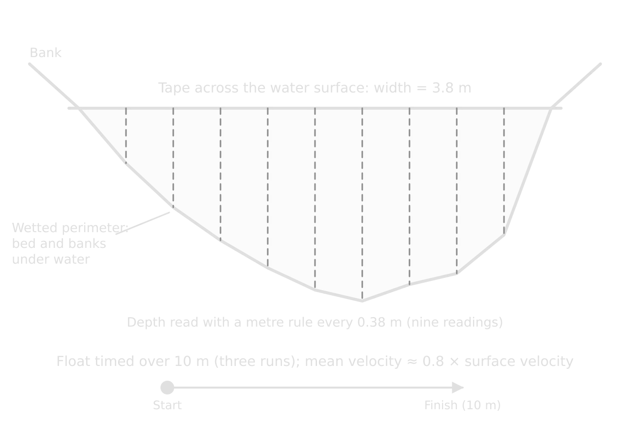
Velocity can be measured with a flow meter, which gives a reading in m s⁻¹ directly, or with a float timed over a measured distance. A float moves at the speed of the surface water, which is faster than the mean, so the surface velocity is multiplied by a correction factor of about 0.8. Three or more runs at each site, averaged, reduce the effect of eddies and timing errors. The wetted perimeter is measured with a chain or a weighted rope laid along the bed from one water edge to the other.
Other channel variables complete the picture. Gradient is measured with a clinometer sighted between two ranging poles a set distance apart (10 m) along the bank. Bedload is sampled by measuring the b-axis (the intermediate axis) of each pebble with callipers, and its roundness is judged against a Powers roundness chart, from very angular to well rounded. Hydraulic radius is calculated as cross-sectional area ÷ wetted perimeter.
Beach profiles
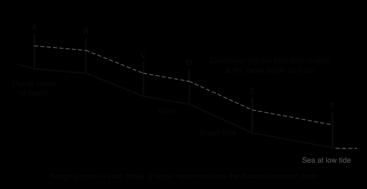
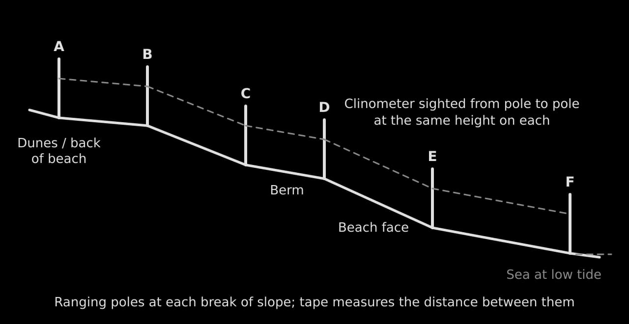
A beach profile measures the shape of a beach from the sea to its landward edge. Two ranging poles are placed at the first break of slope (where the angle of the beach changes); a tape measures the distance between them, and a clinometer, sighted from a mark on one pole to the same height on the other, measures the angle. The poles then leapfrog down the beach to the next break of slope, and the profile is drawn from the distances and angles.
Vegetation and quadrats
Vegetation and ground cover are measured with a quadrat, a square frame (often 0.5 m × 0.5 m, divided into 25 or 100 small squares) placed at intervals along a transect. The percentage of the frame covered by each species, by bare ground or by litter is estimated by counting the small squares. Quadrats along a transect across sand dunes record plant succession; along a footpath, they record trampling.
Questionnaires and interviews
A questionnaire asks a sample of people the same questions in the same order, so that their answers can be counted and compared. Closed questions (tick boxes, yes/no, multiple choice, rating scales) are quick to answer and easy to analyse; open questions give richer, qualitative answers but take longer to process. A Likert scale asks people to rate a statement from "strongly disagree" to "strongly agree" and turns perceptions into numbers.
Keep it short: eight to twelve questions, one side of paper, under three minutes.
Start with easy factual questions (where have you travelled from?) and put sensitive ones (age group) at the end, as ranges.
Avoid leading questions ("Don’t you agree the town is too crowded?") and questions that ask two things at once.
Test it in the pilot study and change any question people misunderstand.
Introduce yourself, explain the purpose and record answers anonymously; respect a refusal.
Interviews are longer conversations with a few people chosen for what they know: a shopkeeper, a council officer, a farmer, a warden. They provide explanations and perspectives that numbers cannot, and they are qualitative evidence to be quoted briefly and compared with the measured data.
Environmental quality surveys
An environmental quality survey scores the quality of a place on a set of criteria, each on a fixed scale between two opposites. Each site is scored on the same criteria, and the scores are totalled into an index that can be compared between sites and presented on a bipolar graph.
Criterion | −3 | −2 | −1 | 0 | +1 | +2 | +3 | Criterion |
|---|---|---|---|---|---|---|---|---|
Litter | A lot of litter | No litter | ||||||
Noise | Very noisy | Quiet | ||||||
Graffiti and vandalism | Widespread | None | ||||||
Green space | None visible | Extensive and well kept | ||||||
Building condition | Derelict | Excellent | ||||||
Traffic | Heavy, congested | Very light |
The scores are subjective: two people may score the same street differently. Reliability improves when the criteria are described precisely (what counts as "a lot of litter"), when two people score each site independently and their scores are averaged, and when all sites are surveyed at the same time of day.
Pedestrian and traffic counts
A pedestrian count records the number of people passing a fixed point in a set time, such as ten minutes, using a tally or a hand counter. Counting at many sites at the same time, with several people, gives a snapshot of how busy each part of a settlement is; repeating counts at different times shows daily and weekly variation. Traffic counts work in the same way and can separate cars, buses, lorries and bicycles.
Land-use mapping, photographs and field sketches
Land use is recorded by walking a route and classifying each building or plot (retail, offices, residential, services, open space, vacant) on a base map, usually the ground floor only. Photographs record evidence at each site and become figures when they are annotated. A field sketch goes further: it selects only the relevant features of a view and labels and annotates them, which shows the investigator’s interpretation.
Recording data accurately
Data are recorded in the field on a recording sheet prepared in advance, with a row for each site and a column for each measurement, units in the headings and space for repeat readings, the time and notes. Writing down raw readings, not calculated values, means mistakes can be found and corrected later. Each site is photographed and its position recorded with GPS or a grid reference.
Site | Time | Width (m) | Depths at 0.1 w intervals (m) | Float times over 10 m (s) | Wetted perimeter (m) | Pebble b-axes (mm) | Notes |
|---|---|---|---|---|---|---|---|
5 | 11:40 | 3.8 | 0.10, 0.18, 0.24, 0.29, 0.33, 0.35, 0.32, 0.30, 0.23 | 20.4, 21.6, 21.2 | 4.43 | 38, 42, 47 … (15 values) | 400 m below the Hollin Gill confluence; dry two days; photo 14 |
The recording sheet holds raw readings only, one row per site, so that every later value can be traced back to what was measured. The notes column records anything that could explain an unusual result, such as a fallen tree, a tributary or livestock in the water.
Two qualities decide how far the data can be trusted. Reliability is whether the method gives consistent results when repeated; validity is whether it measures what the investigation actually needs to know. A float run repeated three times with similar times is reliable; it is valid as a measure of mean velocity only after the correction factor has been applied and if it was released in the main current.
A method can be reliable without being valid. Counting pedestrians for ten minutes at 9 a.m. on a Monday gives consistent results week after week, but it is not a valid measure of how busy a shopping street is on a Saturday.
Bias is a systematic distortion: results pushed in one direction by the way data were chosen, recorded or interpreted. Sampling bias comes from unrepresentative sites or respondents (only measuring where the bank is easy); measurement bias from equipment or habits (always reading the metre rule from above the water, which adds the height of the bow wave); personal bias from expectations (scoring a run-down street lower because it was expected to be poor).
Problem | Effect on data | How to reduce it |
|---|---|---|
Reaction time with a stopwatch | Random error in float times | Longer timing distance; three or more runs; the same person timing |
Metre rule pushed into soft sediment | Depths too large | Rest the rule on the bed surface; read at eye level |
Different people scoring an EQS | Inconsistent scores between sites | Precise criteria; two scorers per site; average the scores |
Questionnaires only on one weekday morning | Some groups over- or under-represented | Survey at different times and days; stratify by age |
River level changing during the day | Sites not comparable | Measure all sites on one day; note rainfall; check a gauge record |
Processing the data
Processing turns raw readings into the values that answer the hypotheses: means of repeat readings, cross-sectional areas, discharges, percentages, index scores. The processed data are best shown in one clear table, with units in every column heading and the same number of decimal places in each column. Such tables of numbers are not counted in the 2,500 words.
Site | Distance from source (km) | Width (m) | Mean depth (m) | Area (m²) | Mean velocity (m s⁻¹) | Discharge (m³ s⁻¹) | Wetted perimeter (m) | Hydraulic radius (m) | Mean pebble b-axis (mm) |
|---|---|---|---|---|---|---|---|---|---|
1 | 0.8 | 1.2 | 0.11 | 0.13 | 0.21 | 0.028 | 1.48 | 0.09 | 112 |
2 | 2.1 | 1.9 | 0.15 | 0.29 | 0.26 | 0.074 | 2.27 | 0.13 | 96 |
3 | 3.4 | 2.6 | 0.19 | 0.49 | 0.31 | 0.153 | 3.06 | 0.16 | 88 |
4 | 4.6 | 2.6 | 0.24 | 0.62 | 0.24 | 0.150 | 3.17 | 0.20 | 81 |
5 | 5.9 | 3.8 | 0.26 | 0.99 | 0.38 | 0.375 | 4.43 | 0.22 | 64 |
6 | 7.2 | 4.3 | 0.31 | 1.33 | 0.42 | 0.560 | 5.04 | 0.26 | 59 |
7 | 8.4 | 4.1 | 0.36 | 1.48 | 0.47 | 0.694 | 4.95 | 0.30 | 47 |
8 | 9.7 | 5.2 | 0.40 | 2.08 | 0.52 | 1.082 | 6.12 | 0.34 | 41 |
The table is the hypothetical data set for the Kerran Beck, used for every graph and test that follows. Even before any graph is drawn, the trends are visible: width, depth, discharge and velocity rise downstream and pebble size falls. The irregularities are visible too: site 4 is no wider than site 3 and slower than site 2, and site 7 is slightly narrower than site 6. Bed gradient, measured with the clinometer, fell from 6.5° at site 1 to 1.0° at site 8.
Presenting the data
Criterion C rewards the most appropriate techniques, used effectively and following conventions. "Appropriate" means the technique suits the type of data and shows the pattern the hypothesis is about: change with distance suits a scatter graph or a located graph on a map; parts of a whole suit a compound bar or pie chart; a comparison of spreads suits box-and-whisker plots. Variety for its own sake earns nothing, and three different graphs of the same variable are no better than one good one.
Data and purpose | Appropriate technique | Less appropriate |
|---|---|---|
Change in a variable with distance along a river, transect or route | Scatter graph with best-fit line; located graphs or proportional symbols on the map | Pie charts for each site |
The shape of a channel or beach | Cross-sections or profiles drawn to scale, side by side on the same scales | A table of depths alone |
Plant cover along a transect | A separate bar graph for each species | |
Spread of measurements at each site | Box-and-whisker plots or dispersion diagrams | Means alone |
Parts of a total (land use, shop types, transport mode) | Compound bar graph; pie charts for one or two places | Line graph |
Scores between opposites (EQS) | Bipolar graph | Pie chart |
Visitors’ origins; flows of people or goods | Flow-line map; desire lines | A list of place names |
Opinions and perceptions | Bar graph of coded responses; selected quotations | Every response printed in full |
Conventions for every figure
Number every figure (Figure 1, Figure 2…) and refer to it in the text by number.
Give each a title that says what it shows, where and when ("Figure 4: Channel width against distance from source, Kerran Beck, 12 March").
Label both axes with the variable and its unit; start bar graph axes at zero; use the same scales when graphs are to be compared.
Add a key where more than one symbol, line or shade is used; maps need a north arrow and a scale.
Place each figure in the body of the report next to the analysis that uses it, never in an appendix.
Annotate where it helps: a short note on a graph or photograph that points out an anomaly or a feature earns more than a separate paragraph.
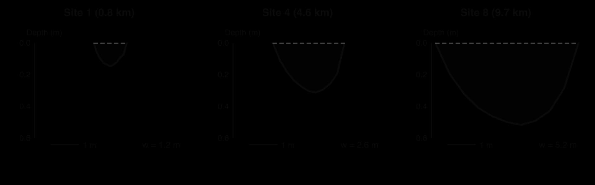
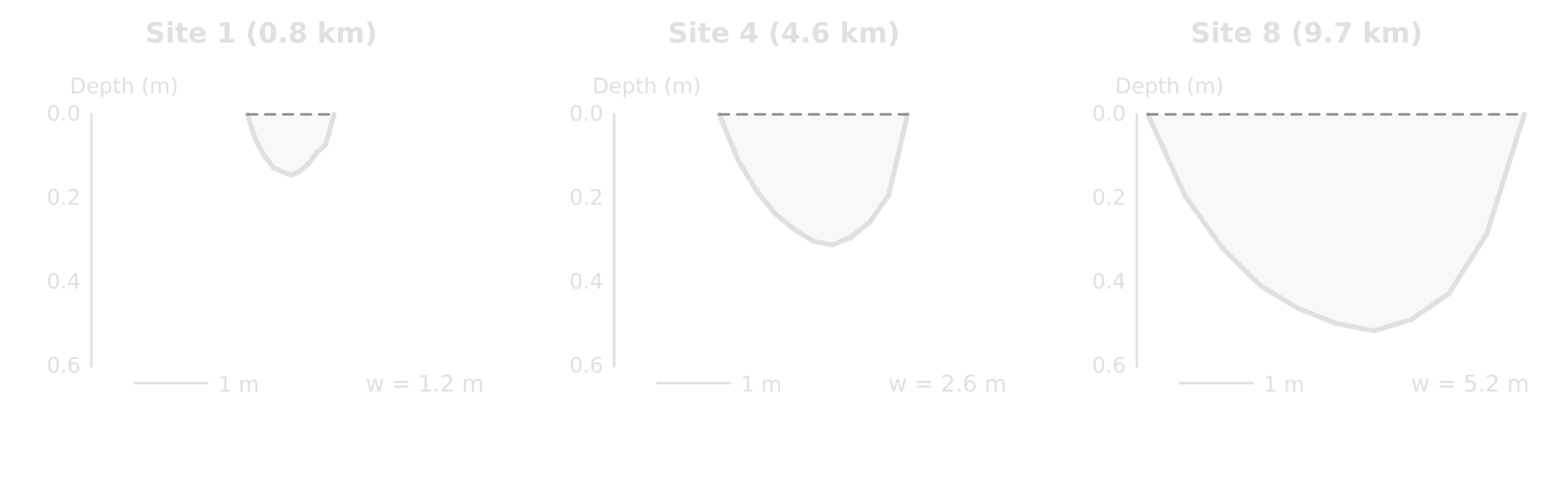
Cross-sections drawn side by side at the same scale are the clearest way to show how the shape of the channel changes. They show something the table does not: at site 4 the channel is as narrow as at site 3 but much deeper, a sign of the pool behind the weir, which matters later in explaining the velocity results.
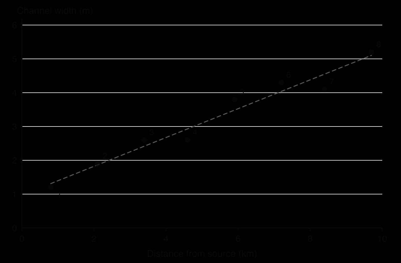
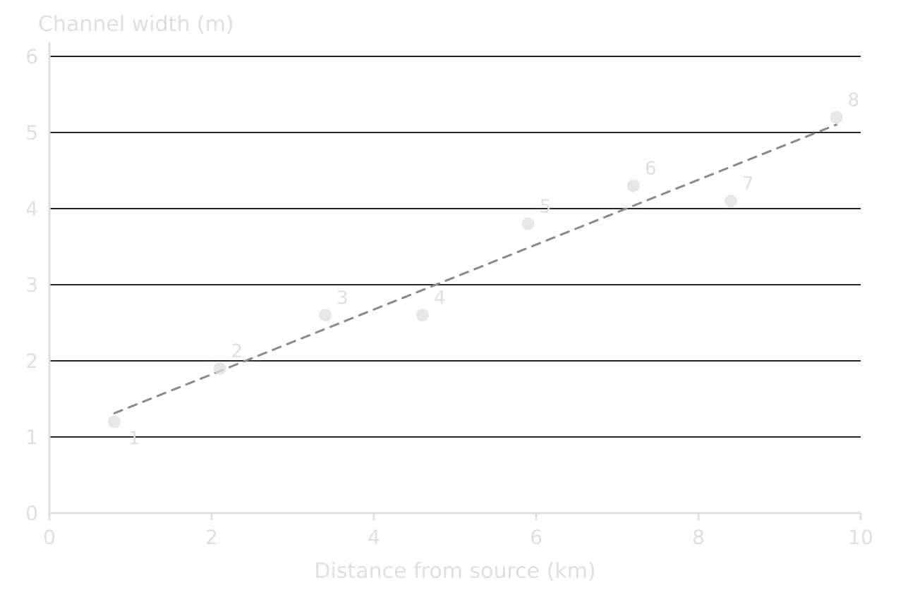
A scatter graph is the most appropriate way to show each hypothesis about change with distance, because distance is a continuous independent variable and the best-fit line shows the trend. The width graph shows a strong positive relationship, the pattern H1 predicts. Spearman’s rank correlation coefficient measures how strong it is and whether it could have arisen by chance.
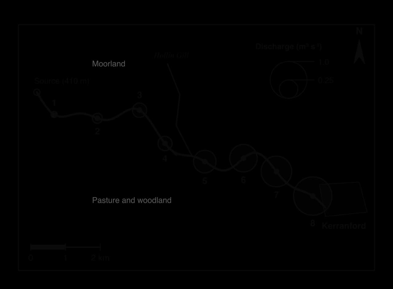
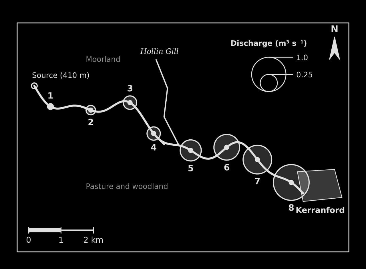
Located data on a map link the results to the place, which is something a graph cannot do. The discharge map shows not only that discharge increases downstream but where it increases most, below the tributary confluence, which supports the explanation that the drainage area and the volume of water collected grow downstream.
A kite diagram from a different investigation
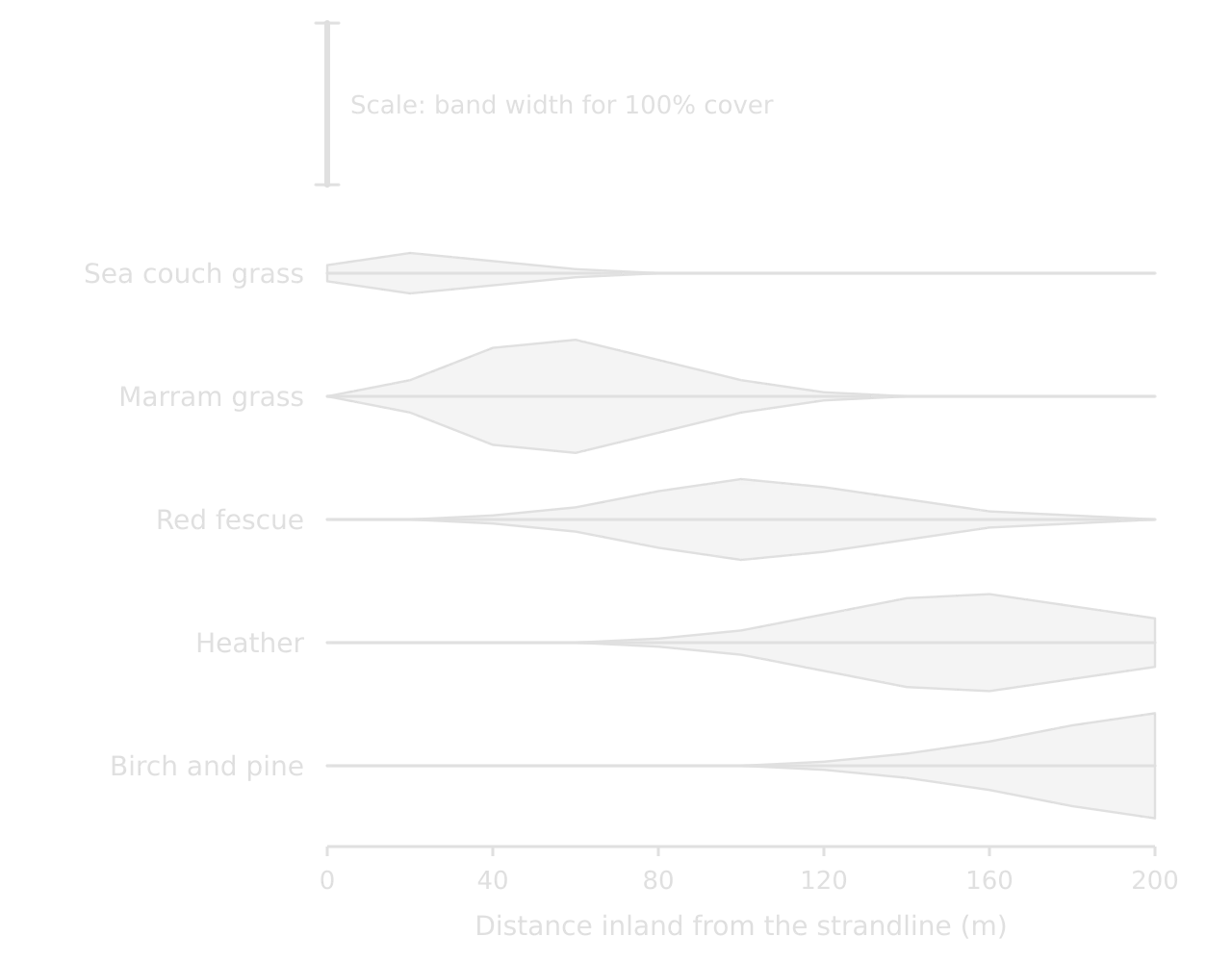
A kite diagram shows how the cover of several species changes along a transect. Each species has its own horizontal axis, and at each sampling point the band is drawn with a width proportional to the percentage cover, half above the axis and half below. It is the standard way to present quadrat data from sand-dune succession or from vegetation either side of a footpath.
Testing relationships: Spearman’s rank
A correlation is a relationship between two variables. Spearman’s rank correlation coefficient () measures its strength and direction using the ranks of the data rather than the values themselves, which makes it suitable for the small samples and uneven data of fieldwork. It ranges from +1 (a perfect positive relationship) through 0 (no relationship) to −1 (a perfect negative relationship).
State the null hypothesis: there is no relationship between the two variables.
Rank each variable separately, 1 for the highest value. Tied values share the mean of the ranks they occupy (two values tied for 5th and 6th each get 5.5). With a few ties the formula still gives a close approximation.
For each pair, find the difference between the ranks (d) and square it (d²).
Add the squared differences (Σd²) and put the total into the formula, with n = the number of pairs.
Compare with the critical value for n at the chosen significance level, and accept or reject the null hypothesis.
Significance and critical values
A correlation coefficient on its own does not show whether a relationship is real or a product of chance: with only a few pairs, a strong-looking value can appear at random. The significance level states how much risk of a chance result is accepted, usually 0.05 (5%, or 95% confidence) or 0.01 (1%, or 99% confidence). The critical value from statistical tables is the coefficient that must be reached for the result to be significant at that level, and it falls as the number of pairs rises.
Number of pairs (n) | One-tailed, 0.05 | One-tailed, 0.01 | Two-tailed, 0.05 | Two-tailed, 0.01 |
|---|---|---|---|---|
8 | 0.643 | 0.833 | 0.738 | 0.881 |
10 | 0.564 | 0.745 | 0.648 | 0.794 |
A one-tailed test is used when the hypothesis predicts the direction of the relationship (width increases downstream); a two-tailed test when it predicts only that there is a relationship. The critical values apply to the size of , so a negative coefficient (such as pebble size against distance) is compared using its absolute value.
Testing differences: the chi-squared test
The chi-squared test compares observed frequencies in categories with the frequencies that would be expected if there were no difference or association. It needs counts (numbers of pebbles, people or shops), never percentages or means, and expected frequencies of at least 5 in each cell.
Choosing a statistical technique
Question about the data | Technique | Data needed |
|---|---|---|
Is there a relationship between two variables measured at the same sites? | Spearman’s rank correlation coefficient | At least 8–10 pairs of values |
Do counts in categories differ from what chance would give, or between places? | Chi-squared test | Frequencies (counts), expected values ≥ 5 |
Are points on a map clustered, random or regular? | Nearest neighbour index | The positions of the points and the area |
Is an activity more concentrated here than in the wider region? | Location quotient | Counts for the area and the reference region |
How do the averages and spreads of two or more samples compare? | Mean, median, interquartile range; box-and-whisker plots | A sample of measurements at each site |
The nearest neighbour index (: 0 clustered, about 1 random, 2.15 regular) and the location quotient (: above 1 means more concentrated than in the reference region) are the other two techniques. In fieldwork they suit questions about the distribution of shops, services or settlements, and about how specialised a town’s economy is.
Collecting and presenting checklist
- To do:
I can name, describe and justify my sampling method and sample size.
- To do:
Each method is described precisely enough to be repeated, with equipment, units, repeats, place and time.
- To do:
My raw data are recorded in the field with units, and processed into one clear table.
- To do:
I can explain how reliable and valid each method is, and what bias it may contain.
- To do:
Every figure is numbered, titled, labelled with units, keyed and referred to in the text.
- To do:
Each hypothesis has the most appropriate graph or map, and the results are located on a map where it helps.
- To do:
I have chosen a statistical test suited to each hypothesis, calculated it correctly and stated its significance level.
- To do:
No figure is in an appendix; the appendix holds at most a sample recording sheet or questionnaire.
Carry on with Geography in Augment
With a free account, Augment remembers where you stopped in the notes and which questions you have marked.