Analysis, conclusion and evaluation

Write an analysis that describes, quantifies and explains patterns and anomalies, a conclusion that answers the fieldwork question, and an evaluation of methods with improvements, then format the report within 2,500 words.

IB Geography
Internal assessment
SL and HL

21 min readLast reviewed 18 Oct 2026

What the written analysis does

The written analysis (criterion D, 8 marks) is the heart of the report and carries almost a third of the marks. It interprets the processed data in relation to the fieldwork question: it describes the trends and spatial patterns, quantifies them with statistics, explains them with geographical theory, and explains the anomalies as well as the general pattern. It is written alongside the graphs and maps, referring to each by number, not as a separate essay after them.

Marks	What an analysis at this level does
1–2	Uses some inappropriate descriptive techniques; outlines the data without linking them to the question; lists only the most obvious trends
3–4	Uses appropriate descriptive techniques; statistics are missing, irrelevant or contain errors; trends are described and linked to the question, which is answered descriptively
5–6	Uses appropriate descriptive and statistical techniques; links trends, patterns and statistics to the question; lists outliers; some gaps in the evidence
7–8	Uses appropriate descriptive and statistical techniques with significance levels; explains trends, patterns, statistics and anomalies, linking them to the question, hypotheses, theory, location and methods; few or no gaps in the evidence

The main difference between the middle and the top bands is explanation. A 5–6 analysis says what the data show and lists the anomalies; a 7–8 analysis says why, using theory, the features of the place and the strengths and limits of the methods, so that every claim in the conclusion is backed by evidence.

A structure for each hypothesis

Taking the hypotheses one at a time gives the analysis a clear structure and makes sure each is answered. For each one, five moves work well, in this order.

Describe the trend or pattern from the figure, with figures and units (the TEA approach: trend, evidence, anomaly).
Quantify it with the statistical test, giving the value, the critical value and the significance level, and say whether the null hypothesis is rejected.
Explain the pattern with geographical theory: the process that produces it.
Explain the anomalies: what makes a site or person depart from the pattern, using what was observed at the site.
Link back to the hypothesis and to the methods: is the hypothesis supported, and how far can the evidence be trusted?

The Kerran Beck analysis

The hypothetical results of the Kerran Beck investigation show how the five moves work. The key processed values for the eight sites are summarised in the first table, and the results of the four Spearman’s rank tests in the second. All four tests use n = 8 pairs; with directional hypotheses, the one-tailed critical values are 0.643 (0.05) and 0.833 (0.01).

Site	1	2	3	4	5	6	7	8
Distance from source (km)	0.8	2.1	3.4	4.6	5.9	7.2	8.4	9.7
Width (m)	1.2	1.9	2.6	2.6	3.8	4.3	4.1	5.2
Discharge (m³ s⁻¹)	0.028	0.074	0.153	0.150	0.375	0.560	0.694	1.082
Mean velocity (m s⁻¹)	0.21	0.26	0.31	0.24	0.38	0.42	0.47	0.52
Hydraulic radius (m)	0.09	0.13	0.16	0.20	0.22	0.26	0.30	0.34
Mean pebble b-axis (mm)	112	96	88	81	64	59	47	41

The second table gives each hypothesis its statistical result, ready to be quoted in the written analysis.

Hypothesis	Variables	Σd²	$r_{s}$	Significance	Decision
H1	Distance and width	2.5	+0.970	Above 0.833: significant at 0.01	H₀ rejected; H1 supported
H2	Distance and discharge	2	+0.976	Above 0.833: significant at 0.01	H₀ rejected; H2 supported
H3	Distance and mean velocity	6	+0.929	Above 0.833: significant at 0.01	H₀ rejected; H3 supported
H4	Distance and mean pebble size	168	−1.000	Above 0.833 (absolute value): significant at 0.01	H₀ rejected; H4 supported

H1 and H2: width and discharge

Channel width increases from 1.2 m at site 1 to 5.2 m at site 8, more than four times wider, and discharge from 0.028 m³ s⁻¹ to 1.082 m³ s⁻¹, almost 39 times greater. Both correlations with distance are very strong and significant at the 0.01 level. The explanation is the growth of the drainage area downstream: every tributary, field drain and spring adds water, and a larger discharge enlarges its channel by eroding the banks and bed.

The pattern is not perfectly regular. The largest single increase in discharge, from 0.150 to 0.375 m³ s⁻¹ (+150%), is between sites 4 and 5, where Hollin Gill joins (shown on the discharge map). This step change is evidence for the explanation: discharge rises fastest where a tributary adds a whole sub-basin’s water at once. Site 7 is slightly narrower than site 6 (4.1 m against 4.3 m) but deeper (0.36 m against 0.31 m), so its cross-sectional area is still larger; at site 7 the channel runs between a stone wall and a tree-lined bank, which resist erosion and keep it narrow.

H3: velocity

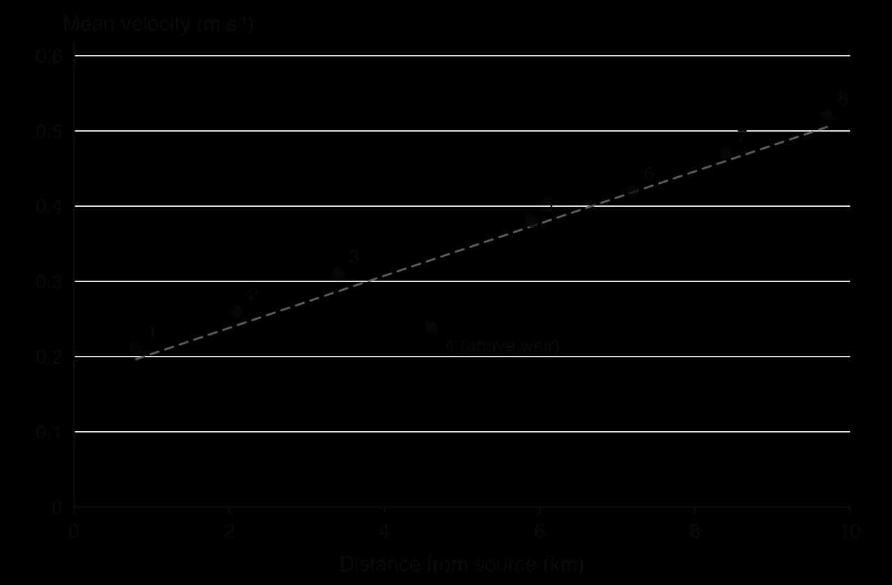
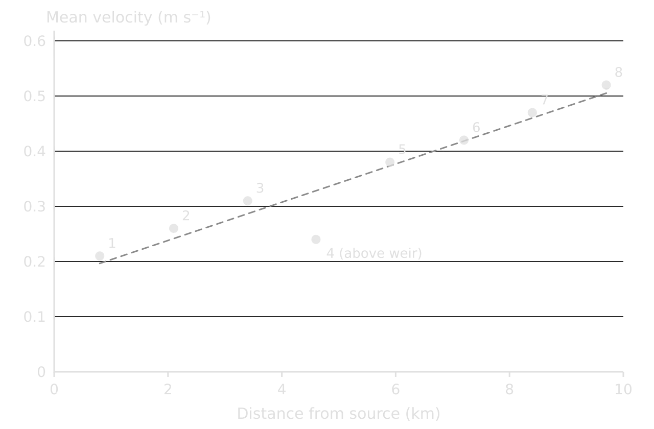
Scatter graph of mean velocity against distance from source: velocity rises from 0.21 m s⁻¹ at site 1 to 0.52 m s⁻¹ at site 8 along a dashed best-fit line; site 4, above a weir, is an anomaly at 0.24 m s⁻¹, below sites 2 and 3. — Mean velocity rises downstream from 0.21 to 0.52 m s⁻¹ along a clear trend. Site 4, 200 m above the weir, is the one anomaly: at 0.24 m s⁻¹ it is slower than sites 2 and 3 upstream. Hypothetical data.

Mean velocity increases from 0.21 m s⁻¹ at site 1 to 0.52 m s⁻¹ at site 8 ( $r_{s}$ = 0.929, significant at the 0.01 level), even though the bed gradient falls from 6.5° to 1.0°. This result supports H3 but contradicts the common expectation that steep mountain streams are faster. The explanation is channel efficiency. Hydraulic radius (cross-sectional area ÷ wetted perimeter) rises from 0.09 m to 0.34 m downstream, so a smaller proportion of the water is in contact with the bed and banks, and less energy is lost to friction. Upstream, the shallow water flows over and around large, angular boulders, which create turbulence and slow the flow.

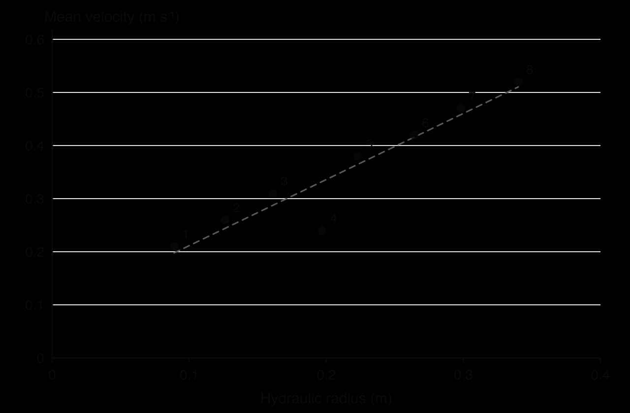
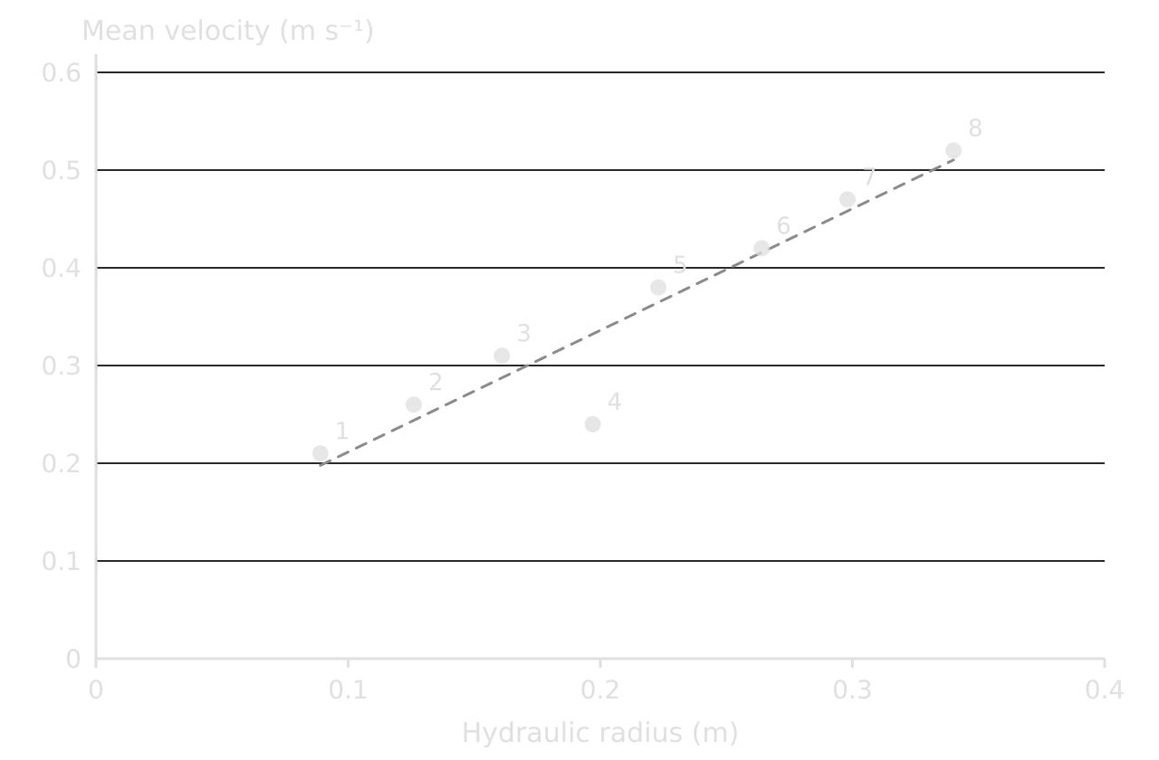
Scatter graph of mean velocity against hydraulic radius for eight sites: hydraulic radius rises from 0.09 to 0.34 m and velocity from 0.21 to 0.52 m s⁻¹; site 4 (R 0.20 m, 0.24 m s⁻¹) lies below the trend. — Velocity rises with hydraulic radius at seven of the eight sites, which supports friction as the explanation. Site 4 again lies well below the trend: its deep pool gives a high hydraulic radius but very slow water. Hypothetical data.

Site 4 is an anomaly in both graphs. It lies 200 m upstream of the weir, which holds back the water and creates a deep, slow pool: the water surface there is almost flat, so the force driving the flow is much smaller than the bed gradient suggests. The anomaly was observed in the field (the pool and the weir are marked on the location map), so it is a real local effect of channel modification, not a measurement error. It also shows a limit of the Bradshaw model, which describes a natural river and does not allow for human structures.

H4: pebble size and shape

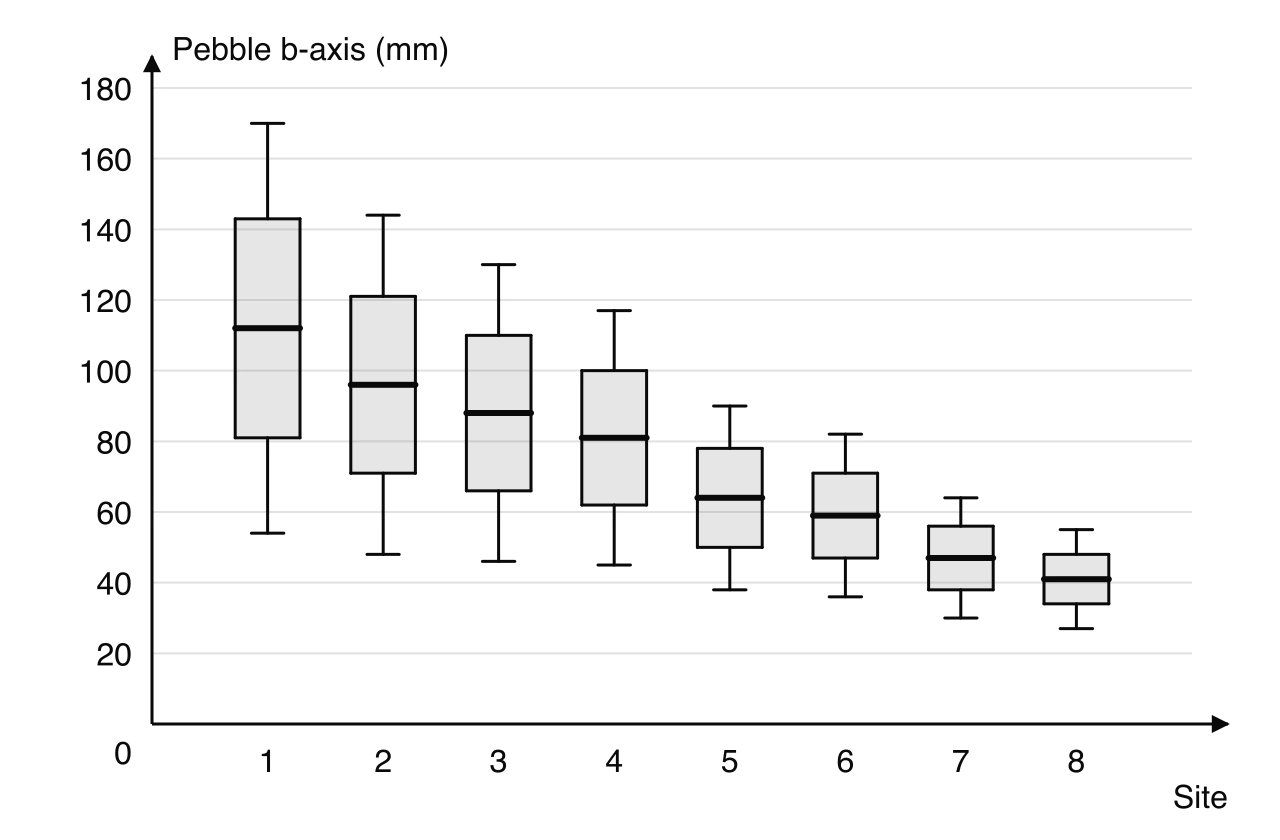
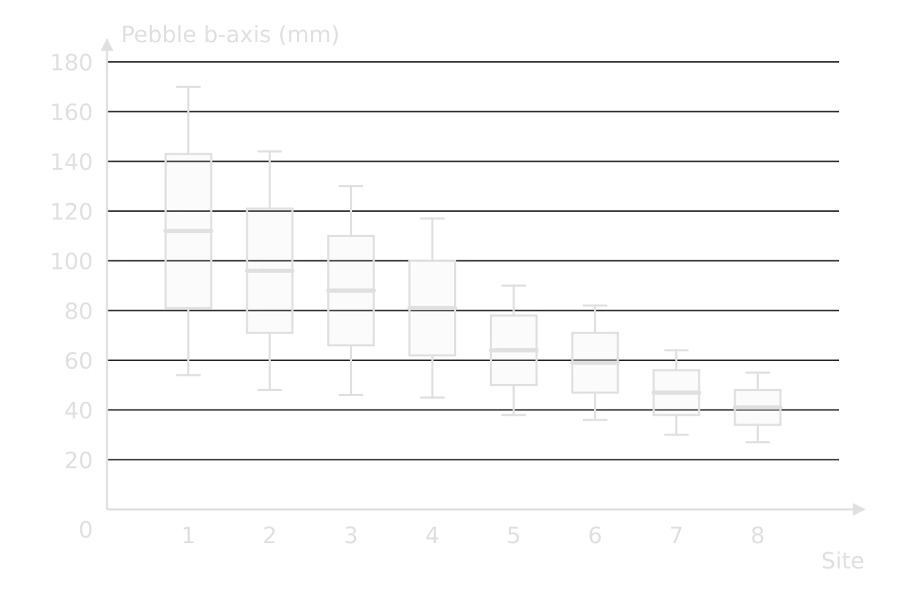
Box-and-whisker plots of pebble b-axis at eight sites, 15 pebbles each: the median falls from 112 mm at site 1 to 41 mm at site 8 and the interquartile range narrows from 62 mm to 14 mm. — The median b-axis falls at every site, from 112 mm to 41 mm, and the interquartile range narrows from 62 mm to 14 mm: downstream, the bedload is smaller and better sorted. Hypothetical data, 15 pebbles per site.

Mean pebble size decreases at every site from 112 mm to 41 mm, a perfect negative rank correlation with distance (Spearman’s rank correlation coefficient $r_{s}$ = −1.000, significant at the 0.01 level). The box-and-whisker plots add that the spread falls too: the interquartile range narrows from 62 mm at site 1 to 14 mm at site 8. Pebbles are also significantly more rounded in the lower course (chi-squared test: χ² = 9.57, df = 3, significant at the 0.05 level).

Two processes can explain the pattern, and the data allow a judgment between them. Attrition and abrasion wear pebbles down and round their edges as they are transported, which explains both the smaller size and the greater roundness. Selective transport also sorts the load: the river moves small particles further and faster than large ones, which would explain the smaller size and better sorting but not, on its own, the change in shape. Since roundness increases as well as size decreasing, wear during transport is likely to be the main process, with sorting adding to it.

Analysing human and qualitative data

The same five moves apply to human geography investigations, with two differences. The patterns often depend on time as well as place (a pedestrian count at 9 a.m. differs from one at noon), and much of the evidence is about perceptions, which need different handling from measurements. Both kinds of data are strongest when they are combined, each checking the other.

A worked example: environmental quality along an urban transect

In a second hypothetical investigation, environmental quality was scored at ten systematic sites every 250 m along a transect from the CBD of a town, using six criteria from −3 to +3 (totals from −18 to +18). The hypothesis was that environmental quality increases with distance from the CBD.

Site	1	2	3	4	5	6	7	8	9	10
Distance from CBD (km)	0.25	0.50	0.75	1.00	1.25	1.50	1.75	2.00	2.25	2.50
EQS total	−10	−8	−6	−7	−2	+1	+3	−4	+6	+11

Using the table of hypothetical data, determine Spearman’s rank correlation coefficient for distance from the CBD and EQS total, test its significance, and suggest an explanation for the anomaly.

Show the solution

Step 1: ranks. Ranking distance (1 = furthest) gives sites 1–10 the ranks 10, 9, 8, 7, 6, 5, 4, 3, 2, 1. Ranking EQS (1 = highest) gives 10, 9, 7, 8, 5, 4, 3, 6, 2, 1.

Step 2: differences. d = 0, 0, 1, −1, 1, 1, 1, −3, 0, 0; d² = 0, 0, 1, 1, 1, 1, 1, 9, 0, 0; Σd² = 14.

r_{s} = 1 - \frac{6 \times 14}{10 \times (10^{2} - 1)} = 1 - \frac{84}{990} = 0.915

Step 3: significance. For n = 10, one-tailed, the critical value at the 0.01 level is 0.745. 0.915 exceeds it, so H₀ is rejected at the 0.01 level: environmental quality increases significantly with distance from the CBD.

Step 4: the anomaly. Site 8 (2.0 km, −4) scores far lower than its neighbours (+3 and +6) and contributes 9 of the 14 in Σd². A suggested explanation is a local feature recorded at the site, such as a busy road junction or a retail park with heavy traffic, noise and litter, which lowers quality regardless of distance from the centre. Field notes or photographs from the site would confirm which.

Questionnaires, interviews and perceptions

Closed questionnaire answers are counted and shown as percentages, graphs or a chi-squared test between groups (for example, whether residents and visitors differ in their views). Open answers and interviews are coded: each answer is sorted into categories (traffic, crowding, cost, safety), the categories are counted, and one or two short quotations illustrate the most common. Each quotation is chosen because it shows a point the analysis makes.

Perceptions need to be compared with measurements, not treated as facts. If 70% of visitors say a footpath is "very crowded" but the visitor count is low, the gap is itself a finding: perceived crowding depends on expectations, and visitors to a remote site expect solitude. Comparing what people say with what was measured, a form of triangulation, is one of the strongest kinds of analysis an integrated investigation can offer.

Writing an analytical paragraph

Two students write about H3. Compare the two paragraphs and identify the band each would reach.

Student A: "Figure 6 shows that velocity goes up as the river goes downstream. Site 8 is the fastest and site 1 is the slowest. Site 4 is an anomaly. This agrees with the Bradshaw model."

Student B: "Mean velocity rises from 0.21 m s⁻¹ at site 1 to 0.52 m s⁻¹ at site 8 (Figure 6), a strong positive correlation with distance ( $r_{s}$ = 0.929, significant at the 0.01 level), so H3 is supported. This happens despite the gradient falling from 6.5° to 1.0°, because hydraulic radius increases from 0.09 m to 0.34 m (Figure 8): less of the water is slowed by friction with the bed. The anomaly at site 4 (0.24 m s⁻¹) lies in the pool behind the weir, where the almost flat water surface reduces the force driving the flow."

Show the commentary

Student A describes the trend without figures, names the anomaly without explaining it, gives no statistic and makes an unexplained link to theory. It is typical of the 3–4 band: trends described and linked to the question, descriptively.

Student B quantifies the trend, gives the statistic with its significance, explains the result with theory (hydraulic radius and friction), links to a second figure, and explains the anomaly from the place. Across all hypotheses, this is the 7–8 band.

Student B’s paragraph is about 95 words and Student A’s about 35. Every extra word in Student B’s paragraph carries evidence or explanation.

Explaining the anomaly well can also strengthen the conclusion. Without site 4, the velocity correlation would be perfect; with it, the analysis shows both the general rule and the local condition that breaks it, which is a more complete answer to the question.

Anomalies and gaps in the evidence

An anomaly is a value that does not fit the general pattern. In the analysis, each one is identified on the graph (an annotation or a label), quantified (how far it lies from the trend) and explained. Anomalies often say more about the place than the trend does: the weir at site 4 shows how far channel modification changes a river’s behaviour.

A gap in the evidence is a claim the data cannot support. The Kerran Beck data show that pebbles become smaller downstream, but because only the b-axis was measured on 15 pebbles at each site, they cannot show how much of the change comes from wear and how much from sorting. A good analysis names such gaps itself, before the marker does, and carries them forward into the evaluation.

The conclusion

The conclusion (criterion E, 2 marks) is a clear, concise answer to the fieldwork question, supported by the analysis. About 200 words are enough. It answers the question directly in its first sentence, states which hypotheses were supported, with the key evidence for each, and notes any important exception. It introduces no new data or ideas; everything in it must already be in the analysis.

A conclusion may find that the results did not match the predictions, and that is a perfectly good conclusion if it is supported by the evidence. What it must not do is claim more than the data show, ignore the hypotheses or end with a sentence that could belong to any report.

Write the conclusion for the Kerran Beck investigation.

Show a model conclusion

Model conclusion. Along the upper 10 km of the Kerran Beck, channel characteristics change downstream largely as the Bradshaw model predicts. Width increased from 1.2 m to 5.2 m and discharge from 0.028 to 1.082 m³ s⁻¹, both significant positive correlations with distance at the 0.01 level, so H1 and H2 are supported; the largest increase in discharge followed the confluence with Hollin Gill.

Mean velocity also increased, from 0.21 to 0.52 m s⁻¹ ( $r_{s}$ = 0.929), supporting H3, because hydraulic radius rose and friction fell even as the gradient decreased. Pebble size decreased at every site ( $r_{s}$ = −1.000) and pebbles became more rounded, supporting H4 and indicating wear during transport. The one clear exception was site 4, where the weir ponded the water and reduced velocity, showing that a human structure can override the natural downstream pattern locally.

Why it earns 2 marks: it answers the question in the first sentence, gives a decision and evidence for each hypothesis, includes the key exception, and every claim comes from the analysis. It is about 140 words.

The evaluation

The evaluation (criterion F, 3 marks) reviews the investigation critically. It explains the strengths and weaknesses of the data collection methods, of the fieldwork question, of the presentation and of the choice of location, and for each important weakness it suggests a specific improvement and explains how the improvement would change the results or the confidence in them. Factors affecting validity and reliability belong here: bias in sampling or scoring, unexpected conditions such as rain the night before, equipment limits and the size of the sample.

Aspect	Strength or weakness	Effect on the results	Improvement and its impact
Sample size	Only eight sites, the minimum for a Spearman test	One unusual site (site 4) has a large effect on $r_{s}$ ; critical values are high	Twelve sites at 0.8 km intervals: a more reliable test and a clearer view of where change happens, including just above and below the confluence
Velocity method	Float timed by hand over 10 m with a 0.8 correction factor	Reaction-time errors; the correction factor is an estimate, so velocity and discharge are approximate	A flow meter at 0.6 of the depth at three points across the channel: a direct mean velocity and more accurate discharge
Timing	All sites measured in one day after two dry days	A strength: sites are comparable; results describe low flow only	Repeat after rain to test whether the pattern holds at higher discharge, which would widen the conclusion
Pebble sampling	15 pebbles per site, chosen by touch	Random and quick; but 15 is a small sample and roundness was judged by eye	Thirty pebbles per site and two people judging roundness independently: smaller random error and less personal bias in the shape data
Location	Sites chosen pragmatically near footpaths	Access points may be at bridges or fords where the channel is modified	Note the channel conditions at each site and avoid sites within 50 m of structures, except to study their effect
Fieldwork question	Focused and testable, but limited to the upper 10 km	The conclusion cannot be extended to the lower course or the floodplain	A second question on the effect of the weir would turn the anomaly into a focus for further study
Presentation	Scatter graphs and located circles are appropriate; but separate velocity and hydraulic-radius graphs show the same anomaly twice	Space and words spent repeating one point	One annotated scatter graph of velocity against hydraulic radius, with site 4 labelled, freeing words for explaining the anomaly

A student writes: "My results could have been more accurate if I had collected more data and used better equipment." Explain why this sentence earns little credit, and rewrite it as a top-band evaluation point.

Show the commentary

Why it earns little: it is generic. It does not say which data or equipment, what was wrong with them, how the results were affected, or what difference the improvement would make. It could be written about any investigation.

Rewritten: "Velocity was measured with a float timed by hand over 10 m, and the three runs at site 1 ranged from 36.5 to 39.6 s, so reaction-time errors were a significant part of each run. Because discharge is calculated from velocity, this error carries into H2. Using a flow meter at 0.6 of the depth would measure mean velocity directly and remove the estimated 0.8 correction factor, so discharge values, and the confidence in H2, would improve, especially at the slow upstream sites where errors are largest."

Formatting the report

The report is easiest to read, and to mark, when its sections follow the criteria. A short title page and a contents page help the marker find each part.

Section	Contents	Criterion
Title page	Fieldwork question, course topic link, candidate code, word count	—
Contents	Section headings and page numbers	—
1. Fieldwork question and geographic context	Question, location and context, theory, hypotheses, location map	A
2. Methods of investigation	Each method described and justified; sampling; time and conditions	B
3. Results and analysis	Processed data table; figures; statistics; analysis by hypothesis, integrated	C and D
4. Conclusion	Answer to the question, by hypothesis	E
5. Evaluation	Strengths, weaknesses, improvements and their impact	F
References	Every source cited, in a standard system	—
Appendix (optional)	A sample recording sheet or questionnaire only	—

Many reports combine criteria C and D in one results section, with each figure followed by its analysis. That is usually the clearest arrangement, because each paragraph of analysis refers directly to the figure it follows and nothing has to be repeated.

The word limit

The limit is 2,500 words, and a moderator reads no further, so a report that runs over loses its conclusion and evaluation, which are the last sections. Knowing what is counted makes it easier to stay within the limit without cutting analysis.

Counted	Not counted
All main text: the question, context, methods, analysis, conclusion and evaluation	Title page, acknowledgements and contents page
Annotations on figures of more than 10 words	Section titles and subtitles
Footnotes of more than 15 words	References, and footnotes of 15 words or fewer
	Map keys and legends; labels of 10 words or fewer
	Tables of statistical or numerical data, or of categories
	Calculations, and appendices containing only raw data or calculations

Figures, references and appendices

Every graph, map, table and photograph is numbered in order and has a title; the text refers to each by number. All figures sit in the body of the report, close to the analysis that uses them, never in an appendix. Pages are numbered. Every source, including base maps, is cited in the text (author, year) and listed in the references, for example: Environment Agency (2024) River gauge data, station 12345. Available at: [URL] (Accessed: 3 March 2026).

Appendices are for very little: one blank or sample recording sheet, or one copy of the questionnaire and its translation if it was used in another language. Completed questionnaires, pages of raw data, secondary material and extra graphs do not belong there, and the marker is not expected to read them.

Why reports lose marks

Criterion	Common weakness	Fix
A	Question too broad, or no precise location; downloaded map without sites or conventions	Name the place and the variables; draw your own map with numbered sites, north arrow, scale, key and inset
A	Long theoretical introduction	Theory in two or three sentences that lead to the hypotheses
B	Equipment listed, methods not justified	For each method: what, how, where, when, how many, and why it tests the hypothesis
C	Graphs without titles, units or numbers; inappropriate graph types	Follow conventions on every figure; choose the technique that shows the pattern in the hypothesis
C	Too little data, or only one or two variables	Enough sites or respondents for a test; several variables that together answer the question
D	Description without explanation; statistics without significance; anomalies ignored	Describe, quantify, explain with theory, explain anomalies, link to methods
E	Conclusion not stated, or not supported	Answer the question in the first sentence; evidence for each hypothesis
F	Generic evaluation; improvements without their impact	Specific weaknesses, their effect on results, and the effect of each improvement
All	Over 2,500 words	Use tables and short annotations; cut description, not analysis

Final checklist

To do:
The fieldwork question is focused, geographical, located precisely and linked to a named course topic and theory.
To do:
Every hypothesis is stated with its null hypothesis, and each is answered in the analysis and the conclusion.
To do:
The location map is my own, with a title, north arrow, scale, key, numbered sites and an inset.
To do:
Each method is described and justified, including sampling, sample size, time and conditions.
To do:
The processed data table has units in every heading; raw data were recorded in the field.
To do:
Every figure is numbered, titled, labelled, keyed, placed in the body and referred to in the text.
To do:
Each statistical test is appropriate, correctly calculated and reported with its critical value and significance level.
To do:
The analysis describes, quantifies and explains each pattern with theory, and explains every anomaly.
To do:
The conclusion answers the question in its first sentence and is supported by the analysis.
To do:
The evaluation explains the most important strengths and weaknesses and the impact of each improvement.
To do:
The main text is no more than 2,500 words, and the appendix holds at most a sample recording sheet or questionnaire.
To do:
Every source is referenced, and the analysis, conclusion and evaluation are entirely my own work.

Carry on with Geography in Augment

With a free account, Augment remembers where you stopped in the notes and which questions you have marked.

Start free