Calculations and data skills

Work through every ESS calculation with correct working, units and rounding, from the Lincoln index to doubling time, and describe trends, read systems diagrams and construct graphs that earn full marks.

IB Environmental Systems and Societies
Exam skills
SL and HL

27 min readLast reviewed 15 Oct 2026

ESS questions use numbers in almost every topic: productivity and energy transfer, population estimates and diversity indices, water budgets, birth and death rates, footprints and changes over time. The calculations themselves are short and use simple arithmetic, but marks are easily lost through missing working, missing units or careless rounding. Data skills, such as describing a trend with values or choosing the right graph, are tested just as often, especially on Paper 1.

Every calculation in the course is set out here with its formula, its units and a worked example, followed by the graph and data skills that go with them. All the data in the worked examples are hypothetical unless a source is given.

Ground rules for every calculation

Calculation questions are usually worth 1–2 marks: one for the working and one for the correct answer with units. A correct final number with no working can lose the working mark, and an answer with no units, or the wrong units, can lose the answer mark. Four habits protect both.

Write the formula in words or symbols before using it.
Substitute the values with their units, so a units error shows up straight away.
Keep full precision until the end, then round the final answer once.
Give the answer with units and, where it helps, a sign or a word: “−35%” or “a decrease of 35%”.

Units

ESS uses SI units and units derived from them. Rates include a unit of time (per year, per day), and quantities measured over an area include a unit of area (per square metre, per hectare). Productivity, for example, is measured in kJ m⁻² yr⁻¹ or g m⁻² yr⁻¹: energy or mass, per square metre, per year. Writing “kJ” alone for a productivity value is incomplete and usually loses the mark.

Quantity	Common units in ESS	Notes
Energy, productivity	kJ m⁻² yr⁻¹; J m⁻² day⁻¹	1 kJ = 1,000 J
Biomass, productivity	g m⁻² yr⁻¹; kg m⁻²; t ha⁻¹	1 ha = 10,000 m²; 1 t = 1,000 kg
Primary productivity (as carbon)	kg C m⁻² yr⁻¹	Mass of carbon fixed
Concentration in water	mg L⁻¹ (≈ ppm in dilute water)	Nitrate, phosphate, dissolved oxygen, BOD
Population density	individuals m⁻²; individuals km⁻²	Per unit area
Birth and death rates	per 1,000 people per year	Crude rates
Water flows	mm yr⁻¹; m³ s⁻¹; km³ yr⁻¹	1 mm of water over 1 m² = 1 litre
Ecological footprint, biocapacity	global hectares (gha) per person	Compare like with like
Carbon footprint	t CO₂-eq	Tonnes of carbon dioxide equivalent

Standard form

Very large and very small numbers are easier to write and compare in standard form: a number between 1 and 10 multiplied by a power of ten. The world population of about 8,200,000,000 in 2025 is 8.2 × 10⁹; a pollutant concentration of 0.000 35 g L⁻¹ is 3.5 × 10⁻⁴ g L⁻¹. To multiply numbers in standard form, multiply the first parts and add the powers: (2 × 10³) × (4 × 10⁵) = 8 × 10⁸.

Significant figures and rounding

An answer should not look more precise than the data it came from. Significant figures are the digits that carry meaning about precision, counted from the first non-zero digit. As a rule, give a calculated answer to the same number of significant figures as the least precise value used, or to the number the question asks for.

Percentages, percentage change and rates

Many Paper 1 calculations are percentages and rates. They look simple, but each has a common trap: dividing by the wrong value.

Percentage of a total

percentage = \frac{part}{total} \times 100

This gives shares: the percentage of a catchment under forest, the percentage of energy passed to the next trophic level, the percentage of quadrats containing a species.

Percentage change

Percentage change compares a change with the starting value. It is positive for an increase and negative for a decrease.

percentage change = \frac{new value - original value}{original value} \times 100

Rate of change

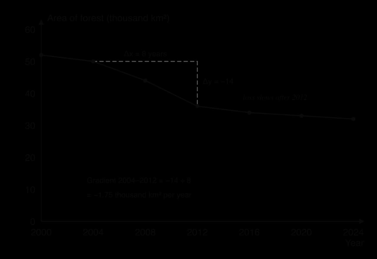
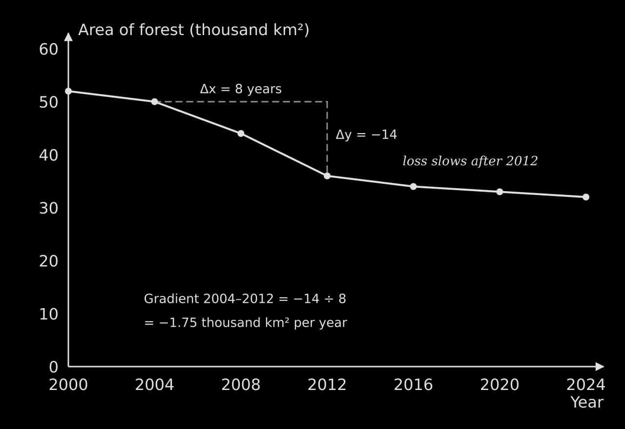
A rate of change divides a change by the time (or distance) over which it happened. It makes changes over different periods comparable: a loss of 20,000 km² of forest in 24 years and 14,000 km² in 8 years are very different rates.

rate of change = \frac{change in quantity}{time taken}

Mean, median and mode

Averages summarise a set of measurements, such as counts in several quadrats. The mean is the total divided by the number of values; the median is the middle value when the values are put in order; the mode is the most frequent value. The median is less affected by an extreme value than the mean. Measures of spread, such as the range, standard deviation and interquartile range, and statistical tests are used mainly in the individual investigation.

Sampling calculations

Ecological fieldwork produces counts from samples, which are scaled up to estimate the whole population or community. Each method has its own calculation, and each estimate rests on assumptions that are worth stating in an evaluation.

Population density, percentage cover and percentage frequency

For plants and other non-motile organisms, counts in quadrats give population density: the number of individuals per unit area. Percentage cover estimates the proportion of a quadrat’s area covered by a species, and percentage frequency is the percentage of quadrats (or squares within a quadrat) in which the species occurs.

population density = \frac{number of individuals counted}{total area sampled}

percentage frequency = \frac{number of quadrats containing the species}{total number of quadrats} \times 100

The Lincoln index

Animals that move are counted by capture–mark–release–recapture. A first sample is caught, marked harmlessly and released; after they have mixed back into the population, a second sample is caught and the marked individuals in it are counted. The Lincoln index uses the proportion of marked individuals in the second sample to estimate the population.

population size = \frac{M \times N}{R}

M = number of individuals caught and marked in the first sample
N = total number caught in the second sample
R = number of marked individuals recaptured in the second sample

Simpson’s reciprocal index

Simpson’s reciprocal index combines species richness (the number of species) and evenness (how equally the individuals are shared among them) into one value of diversity. The formula is given in questions that use it, but the substitution and the interpretation are where marks are won.

D = \frac{N (N - 1)}{\sum n (n - 1)}

N = total number of individuals of all species
n = number of individuals of a single species; Σ means “the sum of” this value for every species

The lowest possible value is 1, when every individual belongs to one species. The higher the value, the more diverse the community. Values can only be compared fairly between samples of the same type of organism, collected in the same way, in similar ecosystems.

Two meadows were sampled with the same number of quadrats. Meadow X had 20, 15, 10, 3 and 2 individuals of five plant species. Meadow Y had 45, 3, 1 and 1 individuals of four species. Calculate D for each and compare their diversity.

Show the working

Meadow X. N = 50, so N(N − 1) = 50 × 49 = 2,450. Σn(n − 1) = (20 × 19) + (15 × 14) + (10 × 9) + (3 × 2) + (2 × 1) = 380 + 210 + 90 + 6 + 2 = 688. D = 2,450 ÷ 688 = 3.56.

Meadow Y. N = 50, so N(N − 1) = 2,450. Σn(n − 1) = (45 × 44) + (3 × 2) + (1 × 0) + (1 × 0) = 1,980 + 6 + 0 + 0 = 1,986. D = 2,450 ÷ 1,986 = 1.23.

Comparison: meadow X is much more diverse. It has more species (5 against 4), but the main difference is evenness: in meadow Y one species makes up 90% of the individuals, which may show a disturbed or heavily managed meadow.

Science Sauce: a step-by-step walk-through of Simpson’s reciprocal index, the same form as the formula here. Watch for how each n(n − 1) term is set out in a table.

Energy, productivity and biomass

Calculations about energy flow use a small set of relationships. All of them follow from the idea that energy is lost, mainly as heat in respiration, at each step.

Gross and net productivity

Gross productivity is the total gain in energy or biomass; net productivity is what remains after respiratory losses. The same relationship holds for producers (primary) and consumers (secondary).

NP = GP - R

Efficiency of energy transfer

The efficiency of transfer between two trophic levels, called ecological efficiency, is the percentage of the energy at one level that is passed to the next. It is typically 10% or less, but it varies widely between ecosystems and organisms.

efficiency of transfer = \frac{energy at the higher trophic level}{energy at the lower trophic level} \times 100

Secondary productivity (HL)

HL students also calculate productivity for consumers. Energy assimilated (gross secondary productivity) is the food eaten minus the energy lost in faeces; net secondary productivity subtracts respiration as well.

GSP = food ingested - faecal loss NSP = GSP - R

Biomass and energy from dry mass

Biomass is measured as dry mass, because the water content of living tissue varies and contains no usable energy. A sample is dried at about 60–80 °C until its mass stops changing. Its energy content can then be found by burning a dried sample in a calorimeter, and scaled up to the area sampled.

Water and soil calculations

Water budgets

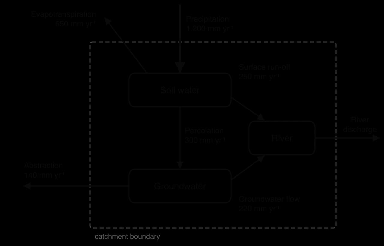
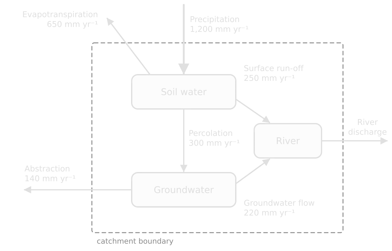
A water budget treats a catchment, lake or aquifer as a system and compares inputs with outputs. If inputs exceed outputs, the storage increases; if outputs exceed inputs, it decreases. Abstraction from an aquifer is sustainable only if it does not exceed the rate of recharge over the long term.

change in storage = inputs - outputs

Systems diagram of a hypothetical catchment. Precipitation 1,200 mm yr⁻¹ enters soil water; evapotranspiration 650 leaves; surface run-off 250 to the river; percolation 300 to groundwater; groundwater flow 220 to the river; abstraction 140 leaves; the river discharges out. — A catchment water budget drawn as a systems diagram (hypothetical values). Arrows leaving the dashed boundary are outputs; comparing the flows into and out of each storage shows whether it is filling or emptying.

Using the water budget in the systems diagram: (a) show that the soil water storage is in balance; (b) calculate the annual change in groundwater storage; (c) the catchment covers 500 km². Convert the groundwater change to a volume in m³.

Show the working

(a) Inputs to soil water = precipitation 1,200 mm yr⁻¹. Outputs = evapotranspiration 650 + surface run-off 250 + percolation 300 = 1,200 mm yr⁻¹. Inputs equal outputs, so the storage is in steady state.

(b) Groundwater input = percolation 300 mm yr⁻¹. Outputs = groundwater flow 220 + abstraction 140 = 360 mm yr⁻¹. Change = 300 − 360 = −60 mm yr⁻¹: the aquifer is being depleted.

(c) 60 mm = 0.06 m; 500 km² = 500 × 10⁶ m² = 5 × 10⁸ m². Volume = 0.06 m × 5 × 10⁸ m² = 3 × 10⁷ m³ per year lost from storage.

Comment: abstraction (140 mm yr⁻¹) is less than recharge (300 mm yr⁻¹), but together with the natural outflow it exceeds recharge, so the current rate is unsustainable.

Biochemical oxygen demand

Biochemical oxygen demand (BOD) is found from two dissolved oxygen readings: one taken immediately and one after the sample has been kept in the dark at 20 °C for five days.

BOD = {DO}_{day 0} - {DO}_{day 5}

Soil water and organic matter

Soil samples are weighed fresh, dried and weighed again to find water content, then heated strongly to burn off the organic matter and weighed a third time. Both percentages are worked out from differences in mass; the organic matter is usually expressed as a percentage of the dry mass.

% water = \frac{fresh mass - dry mass}{fresh mass} \times 100 % organic matter = \frac{dry mass - mass after burning}{dry mass} \times 100

Population calculations

Human population questions use crude rates (per 1,000 people per year), the natural increase rate and the doubling time. The crude rates allow countries of very different sizes to be compared.

CBR = \frac{births in a year}{total population} \times 1,000 CDR = \frac{deaths in a year}{total population} \times 1,000

The natural increase rate is the difference between the crude birth and death rates. It ignores migration. Dividing it by 10 converts it from a rate per 1,000 to a percentage.

NIR (per 1,000) = CBR - CDR NIR (%) = \frac{CBR - CDR}{10}

The doubling time is the number of years a population would take to double if its growth rate stayed the same. It is estimated with the rule of 70.

doubling time (years) \approx \frac{70}{growth rate (%)}

When migration is included, the overall growth rate adds immigration and subtracts emigration. For the same country, with 120,000 immigrants and 40,000 emigrants, growth = (780,000 + 120,000 − 364,000 − 40,000) ÷ 52,000,000 × 100 = 0.95% per year.

Dependency ratio (HL)

The dependency ratio compares the number of people of non-working age with those of working age. A high ratio means each working-age person supports more young or old dependants.

dependency ratio = \frac{population aged 0–14 + population aged 65 and over}{population aged 15–64} \times 100

Footprints, capacity and green GDP

An ecological footprint is sustainable only if it is no larger than the biocapacity available. Both are measured in global hectares (gha), usually per person, so a comparison is a simple subtraction or ratio. Green GDP subtracts the environmental costs of economic activity from GDP.

Green GDP is calculated the same way for any country: the environmental costs are estimated in money terms, which is the difficult and contested part, and then subtracted.

Reading systems diagrams

Systems diagrams appear in every topic, and Paper 1 often gives one with numbers. Reading one is a skill in itself. Boxes are storages; arrows are flows, labelled with the process; arrows crossing the system boundary are inputs or outputs. In a quantitative diagram, the width of an arrow may be drawn in proportion to the size of the flow.

Find the storages and note their units (a store, such as tonnes of carbon or mm of water).
Classify each flow as a transfer (a change of place, such as run-off) or a transformation (a change of state or chemical form, such as evaporation or photosynthesis).
Balance each storage: total inflows minus total outflows gives the change in storage per unit time.
Look for loops: a flow that leads back to its starting storage may be a feedback loop or a cycle.

Graph skills

Choosing a graph

The type of data decides the type of graph. Categories are compared with a bar chart; change over time or along a continuous variable is shown with a line graph; the relationship between two measured variables is shown with a scatter graph.

Graph	Use it for	ESS example
Bar chart	Comparing separate categories	Water footprint of five countries
Histogram	Frequency of continuous data in classes (bars touch)	Number of limpets in each shell-length class
Pie chart	Shares of one whole	Sources of a country’s electricity
Line graph	Change over time or along a continuous variable	Atmospheric CO₂ over 60 years; oxygen downstream of an outfall
Scatter graph	Relationship between two measured variables	Soil moisture against plant height in quadrats
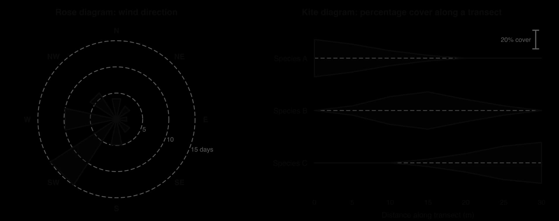
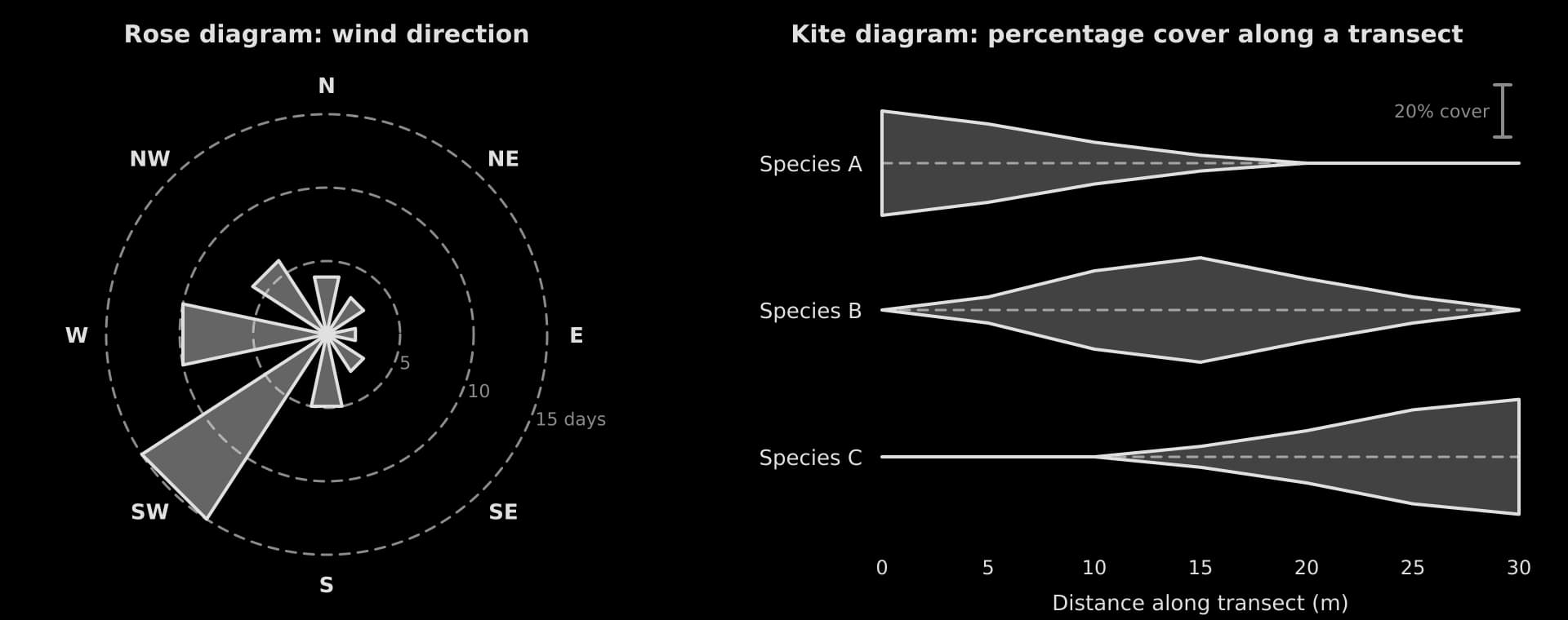
Kite diagram	Abundance of several species along a transect	Zonation on a rocky shore or sand dune
Rose diagram	Directional data	Wind direction; orientation of features
Box and whisker plot	Spread and median of samples, for comparison	Invertebrate counts at two river sites

A histogram looks like a bar chart but shows continuous data grouped into classes, so its bars touch. A pie chart shows the shares of one whole and works only when the parts add up to 100%.

Two specialist graphs are common in ESS fieldwork. A rose diagram shows directional data as bars radiating from a centre. A kite diagram shows how the abundance of several species changes along a transect: the width of each “kite” at any point is proportional to the abundance there.

Left: rose diagram of days of wind from eight directions, with rings at 5, 10 and 15 days; south-west is longest at 15 days, west 10. Right: kite diagram of percentage cover of species A (falls), B (peaks at 15 m) and C (rises) along a 30 m transect. — Left: the longest bar shows the prevailing wind (south-west). Right: the kite widths show species A replaced by B and then C along the transect, the pattern of zonation (hypothetical data).

Constructing a graph

A graph earns marks for its construction as well as its content. The independent variable (the one chosen or controlled, such as time or distance) goes on the x-axis; the dependent variable (the one measured) goes on the y-axis.

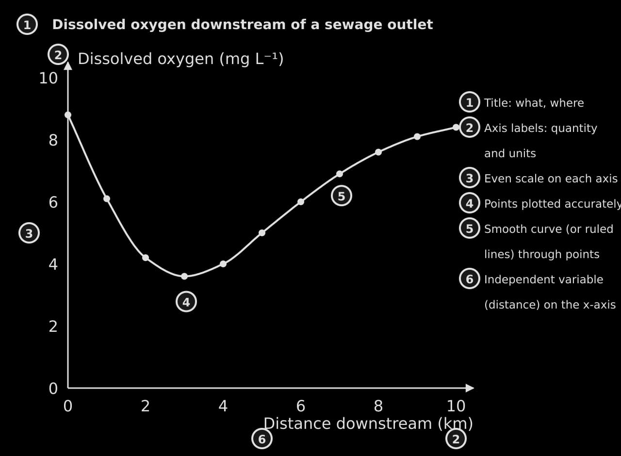
Line graph of dissolved oxygen (mg L⁻¹) against distance downstream of a sewage outlet (km), falling from 8.8 to 3.6 at 3 km and recovering to 8.4 at 10 km. Numbered tags mark title, axis labels with units, even scale, accurate points, smooth curve, x as independent variable. — Six features examiners check on a drawn graph. A missing unit on an axis, or an uneven scale, can cost a mark even when every point is plotted correctly (hypothetical data).

A title that says what is shown, where and when.
Both axes labelled with the quantity and its units.
An even scale on each axis, chosen so the data fill at least half of the grid.
Points plotted accurately, as small crosses or dots.
Points joined with ruled straight lines, or a smooth curve or line of best fit where the relationship is continuous.
A key if there is more than one data set.

Describing trends

A trend description has four parts, in this order: the overall trend, values that support it (with units and dates), any change in the rate, and any anomaly. It does not explain the pattern unless the question asks for reasons.

Line graph of hypothetical forest area, 2000–2024: 52, 50, 44, 36, 34, 33 and 32 thousand km². A dashed triangle from 2004 to 2012 shows Δx = 8 years and Δy = −14, a gradient of −1.75 thousand km² per year; loss slows after 2012. — Forest area falls throughout, but the dashed triangle shows the loss was fastest between 2004 and 2012; afterwards the gradient is much shallower (hypothetical data).

Gradients

The gradient of a line on a graph is the change in the y-value divided by the change in the x-value. On a graph against time, the gradient is the rate of change. A steeper line means a faster change; a curve’s gradient changes along its length.

gradient = \frac{Δ y}{Δ x} = \frac{change in y}{change in x}

Scatter graphs and correlation

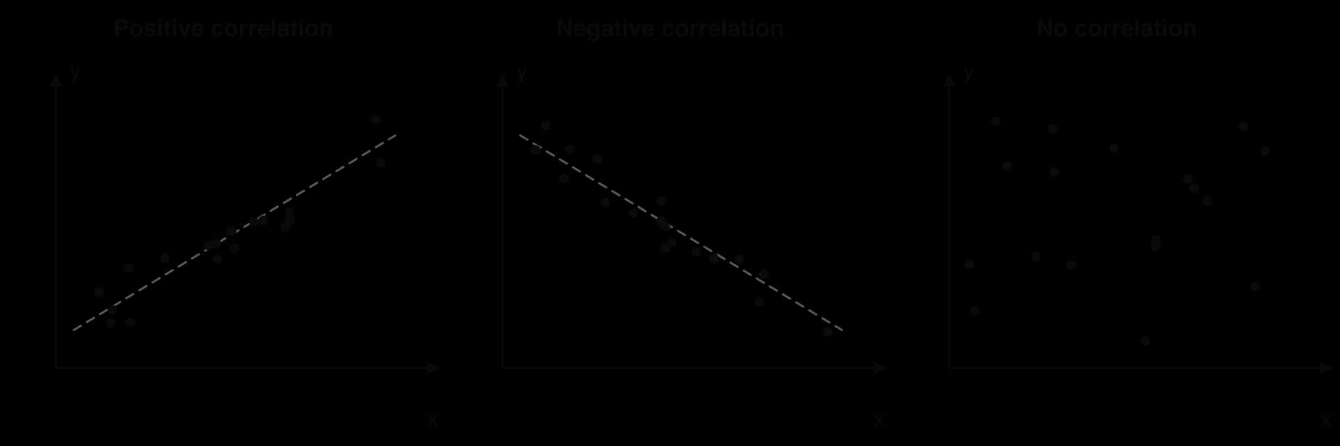
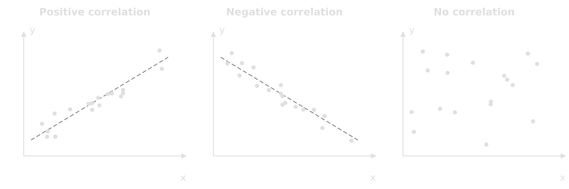
A scatter graph shows whether two variables are related. If both increase together, there is a positive correlation; if one decreases as the other increases, a negative correlation; if the points show no pattern, no correlation. The closer the points lie to a line of best fit, the stronger the correlation.

Three scatter graphs of y against x. Positive correlation: points rise from left to right around a dashed line of best fit. Negative correlation: points fall around a dashed line. No correlation: points scattered with no pattern. — The direction of the line of best fit shows the sign of the correlation; how tightly the points cluster around it shows its strength. The third graph has no line because there is no trend to fit (hypothetical data).

The strength of a correlation is measured with a correlation coefficient, and whether it could have arisen by chance is tested with a statistical test. These tools, and when to use each, belong to data analysis in the individual investigation.

Common calculation mistakes

Unit conversions catch many students too. There are 10,000 m² in a hectare and 1,000,000 m² in a square kilometre; there are 1,000 kg in a tonne. Write the conversion as its own line of working.

Formula summary

Calculation	Formula	Units of the answer
Percentage change	(new − original) ÷ original × 100	%
Rate of change	change ÷ time	quantity per unit time
Population density	number counted ÷ area sampled	individuals m⁻²
Percentage frequency	quadrats with species ÷ total quadrats × 100	%
Lincoln index	M × N ÷ R	individuals
Simpson’s reciprocal index	D = N(N − 1) ÷ Σn(n − 1)	no units (minimum 1)
Net productivity	NP = GP − R	kJ m⁻² yr⁻¹ or g m⁻² yr⁻¹
Efficiency of transfer	energy at higher level ÷ energy at lower level × 100	%
Secondary productivity (HL)	GSP = ingested − faecal loss; NSP = GSP − R	kJ m⁻² yr⁻¹
Water budget	change in storage = inputs − outputs	mm yr⁻¹ or m³ yr⁻¹
BOD	DO on day 0 − DO on day 5 (dark, 20 °C)	mg L⁻¹
Soil water; organic matter	(fresh − dry) ÷ fresh × 100; (dry − burnt) ÷ dry × 100	%
Crude birth or death rate	births or deaths ÷ population × 1,000	per 1,000 per year
Natural increase rate	CBR − CDR (÷ 10 for %)	per 1,000 or %
Doubling time	70 ÷ growth rate (%)	years
Dependency ratio (HL)	(aged 0–14 + aged 65+) ÷ aged 15–64 × 100	dependants per 100
Ecological deficit	footprint − biocapacity	gha per person
Green GDP	GDP − environmental costs	currency
Gradient	Δy ÷ Δx	y-units per x-unit

Carry on with ESS in Augment

With a free account, Augment remembers where you stopped in the notes and which questions you have marked.

Start free