Augment Education
    • Question bank
    • Quick fire
    • Worksheets
    • Flashcards
    • Notes
    • Try a quick-fire round
    • All features
    • Business
    • Digital Society
    • Economics
    • Geography
    • Global Politics
    • History
    • Philosophy
    • Psychology
    • Anthropology
    • World Religions
    • Biology
    • Chemistry
    • Physics
    • Computer Science
    • Design Technology
    • ESS
    • SEHS
    • Language and literature
    • Language acquisition
    • Maths AA
    • Maths AI
    • Dance
    • Film
    • Music
    • Theatre
    • Visual Arts
    • Grade calculator
    • Grade boundaries
    • Subject checker
    • Focus timer
    • Exam countdown
    • All free tools
    • IB guide
    • All subjects
  • Blog

Search

Search subjects, the syllabus, glossary terms, the booklets, the IB guide, help and the blog

Log inStart free
augment

Augment Education

IB Diploma revision built around the syllabus.

contact@augment-education.com

Product

  • Features
  • Question bank
  • Quick fire
  • Worksheets
  • Flashcards
  • Notes
  • Subjects
  • What's new

Learn

  • IB guide
  • Booklets, explained
  • Glossary
  • Blog
  • Free tools
  • Grade calculator
  • Subject checker

Company

  • About
  • Help
  • For parents
  • For teachers
  • Comparisons

Subjects

  • English A Lit
  • English A Lang & Lit
  • Chinese A Lit
  • Chinese A Lang & Lit
  • Spanish A Lit
  • Spanish A Lang & Lit
  • English Lit & Perf
  • Spanish Lit & Perf
  • English B
  • Mandarin B
  • Spanish B
  • English ab initio
  • Mandarin ab initio
  • Spanish ab initio
  • Business
  • Digital Society
  • Economics
  • Geography
  • Global Politics
  • History
  • Philosophy
  • Psychology
  • Anthropology
  • World Religions
  • Biology
  • Chemistry
  • Physics
  • Computer Science
  • Design Technology
  • ESS
  • SEHS
  • Maths AA
  • Maths AI
  • Dance
  • Film
  • Music
  • Theatre
  • Visual Arts

Augment Education is developed independently of the International Baccalaureate Organization and is not endorsed by it. “IB” and “International Baccalaureate” are its trademarks.

© 2026 Augment Education. All rights reserved.

  • Privacy
  • Terms
  1. Subjects
  2. Economics
  3. Quantitative skills and calculations

Quantitative skills and calculations

Work every SL and HL calculation in IB Economics, from PED and real GDP to welfare loss and the multiplier, with the formula, units, a worked example and the traps that cost marks.

  • IB Economics
  • Exam skills
  • SL and HL

48 min readLast reviewed 14 Oct 2026

Economics uses numbers to measure what theory describes: how strongly buyers react to a price change, how fast an economy grows, how much a tax costs society. Every calculation in the course is short, and none needs more than a four-function calculator. Marks are lost on method, units and wording far more often than on difficult arithmetic.

Calculations appear in Paper 2 (part (b) and sometimes parts (c)–(f)), at both SL and HL, and throughout part (a) of HL Paper 3. Paper 1 has no calculator and no calculations. Each calculation is grouped by unit, with what it measures in one sentence, the formula, the units, a fully worked example and the usual traps. HL-only calculations sit under headings marked “(HL only)”.

How calculations are marked

Calculation items are marked with an analytic markscheme: each mark is for a specific step or a specific answer. A typical 2-mark item gives 1 mark for valid working (the formula with the right numbers substituted) and 1 mark for the correct answer with its unit. A 3-mark item usually has a further step, such as finding a percentage change before using it.

Markschemes typically follow your own figures through: if an earlier answer is wrong but the later method is right, the later step can still earn its marks. This only works when the working is written down. A bare number that is wrong earns nothing; a wrong number reached by a visible, correct method usually earns the method mark.

Command term

What it asks for in a calculation item

Calculate

A numerical answer with the relevant steps of working shown.

Determine

The only possible answer, often read from a diagram or a table.

Identify

One answer chosen from the possibilities, such as which country has the comparative advantage.

Plot / Construct

Points marked accurately on a diagram (a Lorenz curve, a PPC) and joined, with labelled axes.

Show that

Working that reaches a result already given in the question; every step must be written.

Comment

A short judgment on the result of the calculation: what it means for the economy or the market.

Exam tip

Write every calculation in three lines: the formula in words or symbols, the formula with the numbers substituted, and the answer with its unit. This takes about 20 seconds longer than writing the answer alone and protects the method mark if the arithmetic slips.

Four habits prevent most lost marks. Give units on every answer ($ billion, thousand units, %, or “no units” for an elasticity). Keep the sign: −0.8 and 0.8 are different answers for a YED. Round only at the end, to two decimal places unless the question says otherwise. Read the scale of each axis and table header, since “$ billion” and “thousand tonnes” change the answer by a factor of a thousand or more.
YouTube
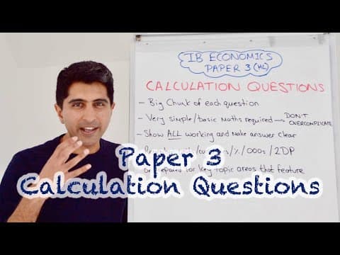
EconplusDal explains how Paper 3 calculation questions are set and marked, and the working examiners look for. The same habits apply to Paper 2 part (b).

All the calculations at a glance

The table lists every calculation in the course by unit. SL students meet the SL rows in Paper 2; HL students meet every row, mostly in Paper 3.

Unit

Calculation

Level

2 Microeconomics

PED; the change in price, quantity demanded or total revenue

SL

2 Microeconomics

YED; the change in income or quantity demanded

SL

2 Microeconomics

PES; the change in price or quantity supplied

SL

2 Microeconomics

Consumer and producer surplus from a diagram

HL

2 Microeconomics

Effects of price ceilings, price floors, indirect taxes and subsidies on markets and stakeholders

HL

2 Microeconomics

Welfare loss from a diagram

HL

2 Microeconomics

Profit, MC, MR, AC and AR from data; concentration ratios

HL

3 Macroeconomics

Nominal GDP (expenditure approach) and nominal GNI

SL

3 Macroeconomics

Real GDP and real GNI with a deflator; real GDP and GNI per capita

SL

3 Macroeconomics

Economic growth rate, unemployment rate, inflation rate from a CPI

SL

3 Macroeconomics

Real interest rate

SL

3 Macroeconomics

Weighted price index; government debt as a percentage of GDP

HL

3 Macroeconomics

Lorenz curve from quintile data; indirect tax paid; total tax and average tax rates

HL

3 Macroeconomics

Keynesian multiplier and the change in GDP; money creation

HL

4 Global economy

Price in another currency; percentage change in a currency’s value

SL

4 Global economy

Balance of payments accounts from data

SL

4 Global economy

Exports, imports, import spending and export revenue from free trade diagrams

HL

4 Global economy

Opportunity costs and comparative advantage

HL

4 Global economy

Effects of tariffs, quotas and production subsidies from diagrams; the Marshall–Lerner sum

HL

Skills every calculation uses

Percentage change

Most calculations in economics are built on percentage change: elasticities, growth rates, inflation rates and exchange rate changes are all percentage changes. It measures how large a change is relative to the starting value, so a $1 rise matters more on a $2 good than on a $200 one.

percentage change=new value−old valueold value×100percentage change=old valuenew value−old value​×100

Worked example

The price of a bus ticket rises from $2.50 to $2.80, and the number of tickets sold falls from 40 000 to 37 000 a day. Calculate the percentage change in the price and in the quantity sold.

Show the solution

Step 1: price. The old value is the price before the change, $2.50.

2.80−2.502.50×100=0.302.50×100=+12%2.502.80−2.50​×100=2.500.30​×100=+12%

Step 2: quantity. The old value is 40 000 tickets.

37 000−40 00040 000×100=−3 00040 000×100=−7.5%4000037000−40000​×100=40000−3000​×100=−7.5%

Answer: the price rises by 12% and the quantity falls by 7.5%. Keep the minus sign: it carries information that later calculations need.

Common mistake

Dividing by the new value instead of the old one. From $2.50 to $2.80 is a 12% rise, but dividing 0.30 by 2.80 gives 10.7%. The base of a percentage change is always the value at the start of the period, unless a question says otherwise.

Percentages and percentage points

When the variable is already a percentage, such as an unemployment rate or an interest rate, two different changes can be described. The difference between the two rates is measured in percentage points; the relative change is a percentage. An unemployment rate that rises from 4% to 6% has risen by 2 percentage points, which is a 50% increase in the rate.

Tip

A quick check: if subtracting two percentages, the answer is in percentage points; if dividing the change by the old rate, the answer is a percentage change. Writing “pp” after a difference keeps the two apart in working.

Reading diagrams and tables

Many HL calculations are areas on a diagram. Surpluses and welfare losses are triangles; tax revenue, subsidy costs and spending are rectangles. Every area in the course is one of these two shapes, or a trapezium that splits into a rectangle and a triangle.

rectangle=width×heighttriangle=12×base×heightrectangle=width×heighttriangle=21​×base×height

On a market diagram the width is a quantity and the height a price, so the area is a sum of money. If quantity is in thousands of units and price in dollars, an area of 75 means $75 000. Read the axis titles before calculating anything.

Unit 2: Microeconomics

Price elasticity of demand (PED)

Price elasticity of demand measures how responsive the quantity demanded of a good is to a change in its price. It has no units, because it divides one percentage by another.

PED=%ΔQd%ΔPPED=%ΔP%ΔQd​​

PED is negative for almost every good, because price and quantity demanded move in opposite directions. It is usually quoted as an absolute value (the minus sign ignored), and its size is what matters: between 0 and 1 demand is price inelastic, above 1 price elastic, and exactly 1 unitary elastic.

Worked example

A café raises the price of a coffee from $3.20 to $3.60. Daily sales fall from 500 to 460 cups. Calculate the PED for coffee at this café, and comment on your answer.

Show the solution

Step 1: percentage change in quantity demanded.

%ΔQd=460−500500×100=−8%%ΔQd​=500460−500​×100=−8%

Step 2: percentage change in price.

%ΔP=3.60−3.203.20×100=+12.5%%ΔP=3.203.60−3.20​×100=+12.5%

Step 3: divide quantity by price. The quantity change goes on top.

PED=−812.5=−0.64PED=12.5−8​=−0.64

Answer: PED = −0.64 (0.64 as an absolute value). Comment: demand is price inelastic, since the quantity demanded falls proportionately less than the price rises. The café’s revenue therefore rises with the price: from $3.20 × 500 = $1 600 to $3.60 × 460 = $1 656 a day.

Questions also give the PED and ask for one of the other values. Rearranging the formula gives the percentage change in quantity demanded: multiply PED by the percentage change in price.

%ΔQd=PED×%ΔP%ΔQd​=PED×%ΔP

Worked example

A concert promoter sells 12 000 tickets at $25 each. PED for the tickets is estimated at −1.5. The promoter cuts the price by 8%. Calculate the new quantity of tickets sold and the change in total revenue.

Show the solution

Step 1: percentage change in quantity demanded. A price cut is a negative change.

%ΔQd=−1.5×(−8%)=+12%%ΔQd​=−1.5×(−8%)=+12%

Step 2: the new quantity. Apply the 12% rise to the old quantity.

12 000×1.12=13 440 tickets12000×1.12=13440 tickets

Step 3: the new price. An 8% cut from $25 is $25 × 0.92 = $23.

Step 4: total revenue before and after. Total revenue is price × quantity.

TR1=25×12 000=$300 000TR2=23×13 440=$309 120TR1​=25×12000=$300000TR2​=23×13440=$309120

Answer: sales rise to 13 440 tickets and total revenue rises by $9 120. This fits the theory: demand is price elastic, so a price cut raises total revenue.

Common mistake

Writing PED with the price change on top. PED = %ΔP ÷ %ΔQd gives −1.56 instead of −0.64 for the coffee, which reverses the conclusion about elasticity. The quantity response is always the numerator: “how much does quantity react, per 1% change in price?”

Income elasticity of demand (YED)

Income elasticity of demand measures how responsive the quantity demanded of a good is to a change in consumers’ income. Unlike PED, its sign matters: positive for a normal good, negative for an inferior good. Above +1 the good is income elastic (often a luxury); between 0 and +1 it is income inelastic (a necessity).

YED=%ΔQd%ΔYYED=%ΔY%ΔQd​​

Worked example

Average household income in a town rises from $40 000 to $44 000 a year. Over the same period, monthly restaurant meals sold rise from 200 000 to 230 000, while sales of instant noodles fall from 1 500 to 1 380 crates. Calculate the YED for each good and identify the type of good.

Show the solution

Step 1: percentage change in income.

%ΔY=44 000−40 00040 000×100=+10%%ΔY=4000044000−40000​×100=+10%

Step 2: restaurant meals. Quantity rises by (230 000 − 200 000) ÷ 200 000 × 100 = +15%.

YEDmeals=+15+10=+1.5YEDmeals​=+10+15​=+1.5

Step 3: instant noodles. Quantity changes by (1 380 − 1 500) ÷ 1 500 × 100 = −8%.

YEDnoodles=−8+10=−0.8YEDnoodles​=+10−8​=−0.8

Answer: restaurant meals have a YED of +1.5, a normal good that is income elastic (a luxury); instant noodles have a YED of −0.8, an inferior good. The sign must be kept in both answers.

Common mistake

Dropping the minus sign on a YED. A YED of 0.8 describes a normal, income-inelastic good; −0.8 describes an inferior good. The two answers lead to opposite conclusions, so a missing sign usually loses the answer mark.

Price elasticity of supply (PES)

Price elasticity of supply measures how responsive the quantity supplied is to a change in the good’s price. It is positive, because quantity supplied rises with price. Above 1 supply is price elastic; below 1 it is price inelastic.

PES=%ΔQs%ΔPPES=%ΔP%ΔQs​​

Worked example

When the price of a crate of tomatoes rises from $50 to $60, growers increase the quantity supplied from 1 000 to 1 150 crates a week. (a) Calculate the PES. (b) Wheat farmers face a PES of 0.4 and currently supply 80 000 tonnes. Calculate the quantity they would supply after a 15% rise in the price of wheat.

Show the solution

(a) Step 1: %ΔQs = (1 150 − 1 000) ÷ 1 000 × 100 = +15%.

Step 2: %ΔP = (60 − 50) ÷ 50 × 100 = +20%.

PES=1520=0.75PES=2015​=0.75

Supply is price inelastic: growers cannot raise output proportionately within a week.

(b) Step 1: rearrange the formula. %ΔQs = PES × %ΔP = 0.4 × 15% = +6%.

80 000×1.06=84 800 tonnes80000×1.06=84800 tonnes

Answer: (a) PES = 0.75; (b) 84 800 tonnes.

The same rearrangement finds any missing value in an elasticity. If YED for restaurant meals is +1.5 and income rises by 4%, quantity demanded rises by 1.5 × 4 = 6%. If PED is −0.5 and a city wants quantity demanded to fall by 10%, the price must rise by −10 ÷ −0.5 = 20%. If PES is 0.75 and quantity supplied rose by 9%, the price must have risen by 9 ÷ 0.75 = 12%.

Tip

Every elasticity in the course has the same shape: the percentage change in quantity on top, the percentage change in the cause (price or income) underneath. Learn one formula and change the denominator.

Consumer and producer surplus (HL only)

HL only

HL students calculate consumer surplus and producer surplus as areas on a market diagram.

Consumer surplus is the difference between what consumers are willing to pay and what they actually pay; producer surplus is the difference between the price producers receive and the lowest price at which they would supply. On a diagram with straight-line curves, each is a triangle.
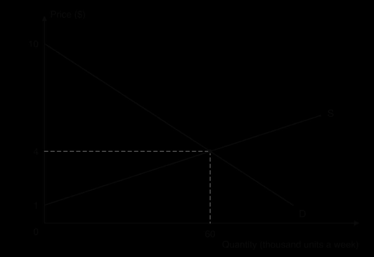
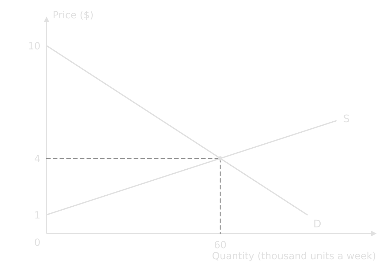
Market diagram: Price ($) against Quantity (thousand units a week). Demand D falls from $10; supply S starts at $1. They cross at a price of $4 and a quantity of 60 thousand.Market diagram: Price ($) against Quantity (thousand units a week). Demand D falls from $10; supply S starts at $1. They cross at a price of $4 and a quantity of 60 thousand.
Market for a good with values on the axes: demand starts at $10, supply at $1, and they cross at $4 and 60 thousand units a week.

Worked example

Using the diagram of the market (quantity in thousand units a week), calculate the consumer surplus and the producer surplus at the equilibrium.

Show the solution

Step 1: identify the triangles. Consumer surplus lies between the demand curve and the price, $4, from 0 to 60 thousand units. Producer surplus lies between the price and the supply curve over the same range.

Market diagram with D from $10 and S from $1 crossing at $4 and 60 thousand units. The triangle between D and $4 is shaded CS; the triangle between $4 and S is shaded PS.Market diagram with D from $10 and S from $1 crossing at $4 and 60 thousand units. The triangle between D and $4 is shaded CS; the triangle between $4 and S is shaded PS.
CS is the triangle above the price and below demand; PS the triangle below the price and above supply.

Step 2: consumer surplus. The base is 60 thousand units; the height is $10 − $4 = $6.

CS=12×60 000×6=$180 000 a weekCS=21​×60000×6=$180000 a week

Step 3: producer surplus. The height is $4 − $1 = $3.

PS=12×60 000×3=$90 000 a weekPS=21​×60000×3=$90000 a week

Answer: CS = $180 000 and PS = $90 000 a week, so social surplus is $270 000.

Common mistake

Using the whole price as the height of the consumer surplus triangle. The height is the gap between where demand meets the price axis and the market price ($10 − $4), not the market price itself.

Price ceilings and price floors (HL only)

HL only

HL students calculate the effects of price controls on the market and its stakeholders: the shortage or surplus, spending, revenue, the cost to the government and the welfare loss.

A price ceiling set below the equilibrium price creates excess demand; a price floor set above it creates excess supply. The quantity actually traded is always the smaller of quantity demanded and quantity supplied. The table gives the demand and supply schedules for the same market.

Price ($)

2

3

4

5

6

Quantity demanded (thousand a week)

80

70

60

50

40

Quantity supplied (thousand a week)

20

40

60

80

100

Worked example

Using the schedules: (a) the government sets a price ceiling of $3. Calculate the shortage, the change in consumer expenditure and the welfare loss. (b) Instead, it sets a price floor of $5 and buys any surplus. Calculate the surplus and the cost to the government.

Show the solution

(a) Step 1: shortage. At $3, Qd = 70 and Qs = 40 thousand. Shortage = 70 − 40 = 30 thousand units.

Step 2: consumer expenditure. Only 40 thousand units are sold, since producers supply no more. Spending falls from $4 × 60 000 = $240 000 to $3 × 40 000 = $120 000: a fall of $120 000 a week. Producer revenue falls by the same amount.

Step 3: welfare loss. The units between 40 and 60 thousand are no longer traded. At 40 thousand, consumers value the last unit at $6 (the demand schedule shows Qd = 40 at $6), while it costs producers $3 to supply.

welfare loss=12×(60 000−40 000)×(6−3)=$30 000welfare loss=21​×(60000−40000)×(6−3)=$30000

(b) Step 1: surplus. At $5, Qs = 80 and Qd = 50 thousand. Surplus = 30 thousand units.

Step 2: cost to the government. It buys 30 000 units at $5: cost = $150 000 a week. Producers now earn $5 × 80 000 = $400 000, while consumers spend $5 × 50 000 = $250 000.

Common mistake

Calculating producer revenue under a price ceiling with the quantity demanded. Firms sell only what they supply, so revenue under a ceiling is the ceiling price × Qs; under a floor, consumer spending is the floor price × Qd.

Indirect taxes (HL only)

HL only

HL students calculate the effects of an indirect tax: tax revenue, the share of the tax paid by consumers and producers, changes in spending and revenue, and the welfare loss.

A specific tax adds a fixed amount per unit to producers’ costs, so the supply curve shifts up by the tax. After the tax, consumers pay the new market price and producers keep that price minus the tax. The diagram shows a $1.50 tax on the same market.
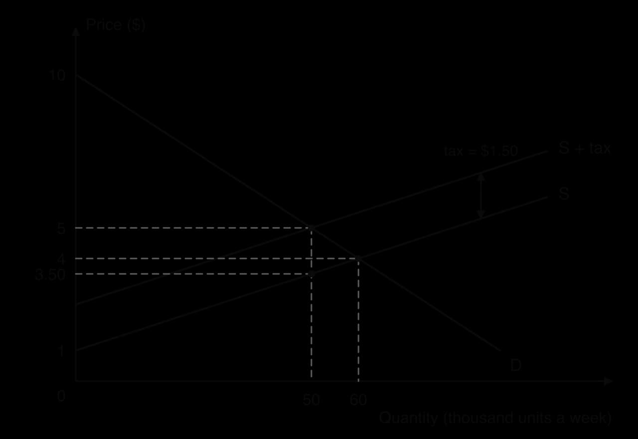
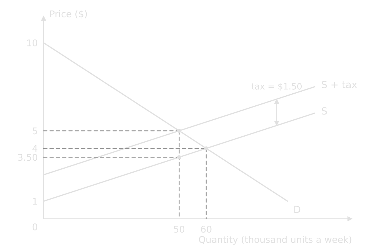
Tax diagram: D, S and S + tax, $1.50 above S. Equilibrium moves from $4 and 60 thousand to $5 and 50 thousand; at 50 thousand units S gives the producer price $3.50.Tax diagram: D, S and S + tax, $1.50 above S. Equilibrium moves from $4 and 60 thousand to $5 and 50 thousand; at 50 thousand units S gives the producer price $3.50.
The tax is the vertical distance between S and S + tax. Consumers now pay $5; producers keep $5 − $1.50 = $3.50; quantity falls to 50 thousand.

Worked example

Using the diagram (quantity in thousand units a week), calculate: (a) government tax revenue; (b) the share of the tax revenue paid by consumers and by producers; (c) the change in consumer expenditure and in producers’ revenue; (d) the welfare loss.

Show the solution
Tax diagram with areas: rectangle A from $4 to $5 and rectangle B from $3.50 to $4, both from 0 to 50 thousand units, form tax revenue. Hatched triangle C between 50 and 60 thousand units is the welfare loss.Tax diagram with areas: rectangle A from $4 to $5 and rectangle B from $3.50 to $4, both from 0 to 50 thousand units, form tax revenue. Hatched triangle C between 50 and 60 thousand units is the welfare loss.
Tax revenue is A + B. A, between $4 and $5, is paid by consumers; B, between $3.50 and $4, by producers. C is the welfare loss.

(a) Tax revenue is the tax per unit × the quantity sold after the tax.

$1.50×50 000=$75 000 a week$1.50×50000=$75000 a week

(b) Tax incidence. Consumers pay $1 more per unit ($5 − $4): $1 × 50 000 = $50 000 (area A, two-thirds). Producers receive $0.50 less ($4 − $3.50): $0.50 × 50 000 = $25 000 (area B, one-third). A + B = $75 000, which checks against (a).

(c) Spending and revenue. Consumer expenditure rises from $4 × 60 000 = $240 000 to $5 × 50 000 = $250 000 (+$10 000). Producers’ revenue, after paying the tax, falls from $240 000 to $3.50 × 50 000 = $175 000 (−$65 000).

(d) Welfare loss is triangle C: the units between 50 and 60 thousand that are no longer traded, with a height equal to the tax.

12×(60 000−50 000)×1.50=$7 500 a week21​×(60000−50000)×1.50=$7500 a week

Tax incidence depends on elasticities: consumers pay the larger share when demand is less elastic than supply, as here. An ad valorem tax is a percentage of the price, so the tax per unit is the rate × the pre-tax price.

Common mistake

Using the old quantity to calculate tax revenue. Revenue is the tax × the quantity sold after the tax (50 thousand), because the tax shrinks the market. $1.50 × 60 000 overstates revenue by $15 000.

Subsidies (HL only)

HL only

HL students calculate the effects of a subsidy: the cost to the government, the gains to consumers and producers, and changes in spending and revenue.

A per-unit subsidy lowers producers’ costs, so supply shifts down by the subsidy. Consumers pay the new, lower market price; producers receive that price plus the subsidy.
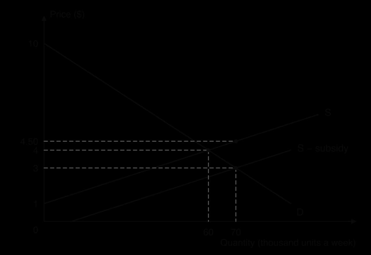
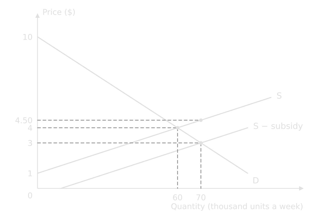
Subsidy diagram: D, S and S − subsidy, $1.50 below S. Price falls from $4 to $3 and quantity rises from 60 to 70 thousand; at 70 thousand units S shows producers receive $4.50.Subsidy diagram: D, S and S − subsidy, $1.50 below S. Price falls from $4 to $3 and quantity rises from 60 to 70 thousand; at 70 thousand units S shows producers receive $4.50.
A $1.50 subsidy shifts supply down to S − subsidy. Consumers pay $3; producers receive $3 + $1.50 = $4.50; quantity rises to 70 thousand.

Worked example

Using the diagram, calculate the cost of the subsidy to the government, the change in consumer expenditure and the change in producers’ revenue.

Show the solution

Step 1: cost to the government = subsidy per unit × new quantity.

$1.50×70 000=$105 000 a week$1.50×70000=$105000 a week

Step 2: consumer expenditure falls from $4 × 60 000 = $240 000 to $3 × 70 000 = $210 000: −$30 000.

Step 3: producers’ revenue, including the subsidy, rises from $240 000 to $4.50 × 70 000 = $315 000: +$75 000.

Step 4: check. Of the $1.50 per unit, consumers gain $1 (the price falls from $4 to $3) and producers $0.50 (they receive $4.50 instead of $4), so consumers get two-thirds of the subsidy, as with the tax.

Welfare loss from externalities (HL only)

HL only

HL students calculate the welfare loss caused by an externality from a diagram.

Where an externality exists, the market produces where private costs equal private benefits, not where marginal social cost equals marginal social benefit. The welfare loss is the triangle between the social curves, from the socially optimal quantity to the market quantity.
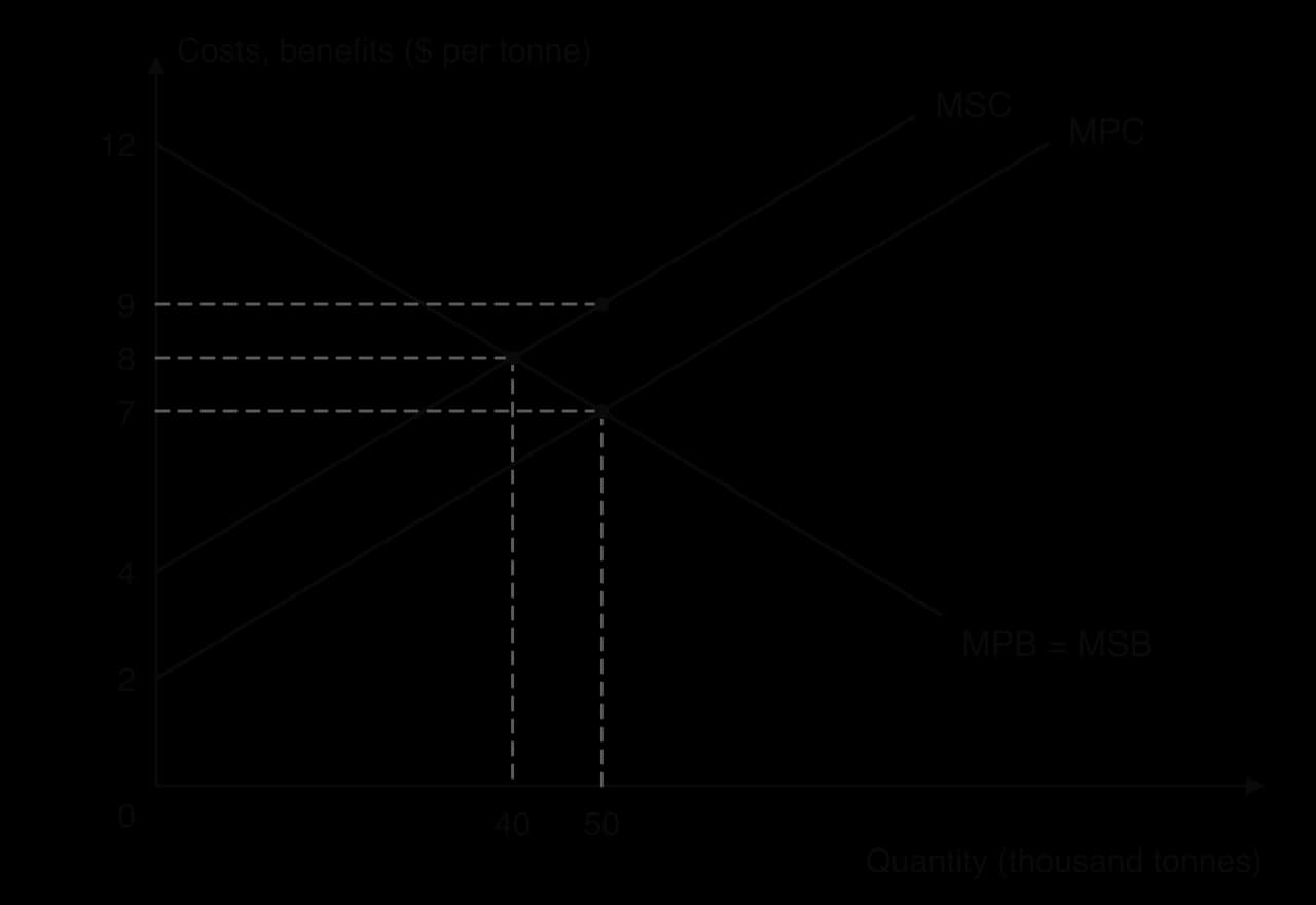
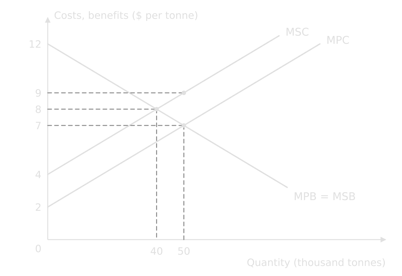
Negative production externality: MPB = MSB falls from $12; MPC starts at $2 and MSC at $4, $2 higher. Market equilibrium at $7 and 50 thousand tonnes; social optimum at $8 and 40 thousand tonnes; MSC at 50 thousand tonnes is $9.Negative production externality: MPB = MSB falls from $12; MPC starts at $2 and MSC at $4, $2 higher. Market equilibrium at $7 and 50 thousand tonnes; social optimum at $8 and 40 thousand tonnes; MSC at 50 thousand tonnes is $9.
Production creates an external cost of $2 a tonne, so MSC lies $2 above MPC. The market produces 50 thousand tonnes; the social optimum is 40 thousand.

Worked example

Using the diagram, calculate the welfare loss caused by the negative externality of production.

Show the solution
The same externality diagram with the welfare loss hatched: the triangle between MSC and MSB from 40 to 50 thousand tonnes, with corners at (40, $8), (50, $9) and (50, $7).The same externality diagram with the welfare loss hatched: the triangle between MSC and MSB from 40 to 50 thousand tonnes, with corners at (40, $8), (50, $9) and (50, $7).
The welfare loss is the hatched triangle: units from 40 to 50 thousand tonnes whose social cost is higher than their social benefit.

Step 1: find the two quantities. The market produces where MPB = MPC: 50 thousand tonnes. Society’s optimum is where MSB = MSC: 40 thousand tonnes.

Step 2: the height of the triangle is the gap between MSC and MSB at the market quantity: $9 − $7 = $2 (the external cost per tonne).

welfare loss=12×(50 000−40 000)×2=$10 000welfare loss=21​×(50000−40000)×2=$10000

Answer: $10 000. The triangle points towards the socially optimal quantity, where MSB = MSC.

Common mistake

Taking the whole area between MSC and MPC as the welfare loss. That parallelogram is the total external cost of the output produced. The welfare loss is only the triangle for the overproduced units, between Q_opt and the market quantity.

Costs, revenues and profit (HL only)

HL only

HL students calculate profit, marginal cost (MC), marginal revenue (MR), average cost (AC) and average revenue (AR) from data, and find the profit-maximising output.

A firm maximises profit where marginal cost equals marginal revenue. The definitions all follow from total revenue (TR) and total cost (TC).

AR=TRQMR=ΔTRΔQAC=TCQMC=ΔTCΔQprofit=TR−TCAR=QTR​MR=ΔQΔTR​AC=QTC​MC=ΔQΔTC​profit=TR−TC

The table gives the prices and total costs of a firm with market power (output in units a day, money in $ thousand).

Output (Q)

0

1

2

3

4

5

6

Price (P)

20

18

16

14

12

10

8

Total cost (TC)

10

16

20

25

32

41

52

Worked example

A firm with market power faces the prices and costs in the table (output in units a day, money in $ thousand). Calculate TR, MR, MC and profit at each output, identify the profit-maximising output, and calculate AC and AR there.

Show the solution

Step 1: TR = P × Q at each output, then MR and MC as the change from the previous row (ΔQ = 1).

Q

0

1

2

3

4

5

6

TR

0

18

32

42

48

50

48

MR

–

18

14

10

6

2

−2

MC

–

6

4

5

7

9

11

Profit (TR − TC)

−10

2

12

17

16

9

−4

Step 2: profit-maximising output. Up to the third unit MR is above MC (10 > 5), so each unit adds to profit. The fourth unit adds MR = 6 but costs MC = 7, so it lowers profit. Output is 3 units, where profit is highest at $17 000.

Step 3: AR and AC at Q = 3. AR = 42 ÷ 3 = $14 thousand (equal to the price). AC = 25 ÷ 3 = $8.33 thousand.

Step 4: check. Abnormal profit = (AR − AC) × Q = (14 − 8.33) × 3 = $17 thousand, matching TR − TC.

Since AR is above AC, the firm earns abnormal profit. Where AR equals AC it earns normal profit, and where AR is below AC it makes a loss.

Common mistake

Dividing total cost by total output to find MC. TC ÷ Q is average cost. MC is the change in total cost divided by the change in output: when output rises in steps of 10, divide the change in TC by 10, not by the new level of output.

Concentration ratios and payoff matrices (HL only)

HL only

HL students also read market structure from data: a concentration ratio and the outcome of a simple game theory payoff matrix.

A concentration ratio is the combined market share of the largest firms in an industry. A four-firm ratio (CR4) adds the shares of the four biggest firms. If the four largest supermarket chains hold 31%, 24%, 12% and 9% of sales, CR4 = 31 + 24 + 12 + 9 = 76%, a high figure typical of oligopoly.

A payoff matrix shows each firm’s profit for every combination of strategies. In the matrix, two firms each choose a high or a low price; each cell shows (Firm A’s profit, Firm B’s profit) in $ million.

Firm B: high price

Firm B: low price

Firm A: high price

(10, 10)

(4, 13)

Firm A: low price

(13, 4)

(6, 6)

Worked example

Using the payoff matrix, identify each firm’s dominant strategy and the likely outcome, and explain why the firms have an incentive to collude.

Show the solution

Step 1: Firm A’s best response. If B prices high, A earns 10 with high and 13 with low, so low is better. If B prices low, A earns 4 with high and 6 with low, so low is better again. Low is A’s dominant strategy.

Step 2: Firm B. The matrix is symmetrical, so low is also B’s dominant strategy.

Step 3: outcome. Both choose low and earn $6 million each, although both would earn $10 million if both priced high. This is a prisoner’s dilemma: collusion on a high price would raise both profits, but each firm then has an incentive to cheat and earn $13 million.

Unit 3: Macroeconomics

Nominal GDP and GNI

Gross domestic product measures the total value of final goods and services produced within a country in a year. The expenditure approach adds the four components of spending on domestic output.

GDP=C+I+G+(X−M)GDP=C+I+G+(X−M)

Gross national income measures the income earned by a country’s residents, wherever their factors of production are located. It adds net income from abroad: income earned abroad by residents minus income paid to non-residents.

GNI=GDP+income from abroad−income paid abroadGNI=GDP+income from abroad−income paid abroad

The table gives national income data for Country A in 2024 (all figures in $ billion, current prices).

Item

$ billion

Consumption (C)

620

Investment (I)

180

Government spending (G)

240

Exports (X)

310

Imports (M)

290

Income earned abroad by residents

45

Income paid to non-residents

70

Worked example

Use the data for Country A in 2024 (all figures in $ billion, current prices) to calculate nominal GDP and nominal GNI.

Show the solution

Step 1: GDP. Net exports are X − M = 310 − 290 = 20.

GDP=620+180+240+20=$1 060 billionGDP=620+180+240+20=$1060 billion

Step 2: GNI. Net income from abroad is 45 − 70 = −25.

GNI=1 060+45−70=$1 035 billionGNI=1060+45−70=$1035 billion

Answer: GDP = $1 060 billion; GNI = $1 035 billion. GNI is lower because foreign owners of firms in Country A earn more there than its residents earn abroad.

Common mistake

Adding imports instead of subtracting them, or leaving out income items that a data table includes as distractors. Only the four spending components enter GDP; the income flows enter GNI only.

Real GDP, real GNI and per capita values

Nominal values are measured at current prices, so they rise with inflation even when output does not. Real GDP removes the effect of price changes using a price deflator, an index of the price level with a value of 100 in the base year.

real GDP=nominal GDPprice deflator×100real GDP=price deflatornominal GDP​×100

The same formula turns nominal GNI into real GNI. Dividing a real value by the population gives a per capita value, a better guide to the average standard of living.

Worked example

Country A’s nominal GDP was $980 billion in 2023 and $1 060 billion in 2024. The GDP deflator was 105 in 2023 and 112.5 in 2024. The population was 52.0 million in 2023 and 52.4 million in 2024. Calculate real GDP and real GDP per capita in both years, and the real GNI in 2024 (nominal GNI $1 035 billion).

Show the solution

Step 1: real GDP.

2023:980105×100=$933.33 bn2024:1 060112.5×100=$942.22 bn2023:105980​×100=$933.33 bn2024:112.51060​×100=$942.22 bn

Step 2: real GDP per capita. Convert both figures to the same units: $942.22 billion ÷ 52.4 million.

2023:933.33×10952.0×106=$17 9492024:942.22×10952.4×106=$17 9812023:52.0×106933.33×109​=$179492024:52.4×106942.22×109​=$17981

Step 3: real GNI in 2024. 1 035 ÷ 112.5 × 100 = $920 billion.

Answer: nominal GDP rose by 8.2%, but real GDP by only about 1%, and real GDP per capita by less than 0.2%. Almost all of the nominal rise was inflation.

Tip

A billion divided by a million is a thousand. So $942.22 billion ÷ 52.4 million = (942.22 ÷ 52.4) × 1 000 = $17 981. Working with the leading numbers and then fixing the scale avoids calculator overflow and dropped zeros.

The rate of economic growth

Economic growth is measured as the percentage change in real GDP over a period, usually a year. Real values are used so that inflation is not counted as growth.

growth rate=real GDPyear 2−real GDPyear 1real GDPyear 1×100growth rate=real GDPyear 1​real GDPyear 2​−real GDPyear 1​​×100

For Country A, growth in 2024 = (942.22 − 933.33) ÷ 933.33 × 100 = 0.95%. The same formula applied to nominal GDP gives 8.16%, which overstates growth because it includes the rise in prices. If a question gives a real GDP index or real GDP directly, no deflating is needed.

Common mistake

Calculating growth from nominal GDP when the data give both. Growth refers to real output. A question that gives only nominal values and a deflator expects the values to be deflated first.

The unemployment rate

The unemployment rate is the percentage of the labour force that is unemployed. The labour force is everyone in work plus everyone actively looking for work; people who are neither (students, retired people, those not seeking work) are left out.

unemployment rate=number unemployedlabour force×100labour force=employed+unemployedunemployment rate=labour forcenumber unemployed​×100labour force=employed+unemployed

Worked example

In Country A, 28.6 million people are employed, 1.9 million are unemployed and actively seeking work, and 12 million adults are outside the labour force. Calculate the unemployment rate.

Show the solution

Step 1: labour force = 28.6 + 1.9 = 30.5 million. The 12 million outside the labour force are not included.

1.930.5×100=6.23%30.51.9​×100=6.23%

Answer: 6.23%. Dividing by the whole adult population (42.5 million) would give 4.47%, a common error.

The inflation rate from a consumer price index

Inflation is a sustained rise in the general price level, measured by the consumer price index. A CPI prices a fixed basket of goods, with quantities that reflect what a typical household buys, so goods bought in larger quantities carry more weight. The index is the cost of the basket in a year relative to the base year; the inflation rate is the percentage change in the index.

price index=cost of basket in the yearcost of basket in the base year×100price index=cost of basket in the base yearcost of basket in the year​×100

The table shows a simple basket of three items, with the quantities a typical household buys and their prices in 2023 and 2024.

Item

Quantity bought

Price 2023 ($)

Price 2024 ($)

Bread (loaves)

100

2.00

2.20

Bus journeys

40

1.50

1.80

Cinema tickets

4

12.00

12.60

Worked example

A simple basket has three items. Using 2023 as the base year, calculate the CPI for 2024 and the inflation rate between 2023 and 2024.

Show the solution

Step 1: cost of the basket in each year. Multiply each price by its quantity and add.

2023:(100×2.00)+(40×1.50)+(4×12.00)=200+60+48=$3082023:(100×2.00)+(40×1.50)+(4×12.00)=200+60+48=$308
2024:(100×2.20)+(40×1.80)+(4×12.60)=220+72+50.40=$342.402024:(100×2.20)+(40×1.80)+(4×12.60)=220+72+50.40=$342.40

Step 2: the index. 2023 is the base year, so its index is 100.

CPI2024=342.40308×100=111.17CPI2024​=308342.40​×100=111.17

Step 3: inflation rate = (111.17 − 100) ÷ 100 × 100 = 11.17%.

Between two years that are not the base year, the inflation rate is still the percentage change in the index. If the index rises from 111.17 to 115.52, inflation is (115.52 − 111.17) ÷ 111.17 × 100 = 3.91%, not 115.52 − 111.17 = 4.35 percentage points.

Common mistake

Averaging the percentage price changes of the goods without weights. Bread rose 10%, bus journeys 20% and cinema tickets 5%; the simple average is 11.67%, but the basket’s cost rose 11.17%, because the goods are bought in different quantities.

The real interest rate

The real interest rate measures the return on saving, or the cost of borrowing, after allowing for inflation. It is approximately the nominal interest rate minus the inflation rate.

real interest rate≈nominal interest rate−inflation ratereal interest rate≈nominal interest rate−inflation rate

With a nominal rate of 5.25% and inflation of 3.4%, the real rate is 5.25 − 3.4 = 1.85%. With a nominal rate of 4% and inflation of 7.5%, it is −3.5%: savers lose purchasing power and borrowers gain. The answer is in percent and can be negative.

Weighted price indices (HL only)

HL only

HL students also calculate a weighted price index in which each category’s weight is its share of household spending.

Official price indices weight each category of spending by its share of the household budget, so a 10% rise in housing costs matters more than a 10% rise in the price of books. Given a price index for each category and its weight, the overall index is the weighted average of the category indices.

weighted index=∑(weight×category index)∑weightsweighted index=∑weights∑(weight×category index)​

The table gives the weight of each category in household spending and its price index for 2024 (base year 2023 = 100).

Category

Weight (% of spending)

Price index 2024

Food

30

108

Housing

40

104

Transport

20

112

Other

10

101

Worked example

Calculate the weighted price index for 2024 (base year 2023 = 100) and the inflation rate.

Show the solution

Step 1: multiply each index by its weight. 30 × 108 = 3 240; 40 × 104 = 4 160; 20 × 112 = 2 240; 10 × 101 = 1 010.

Step 2: add and divide by the sum of the weights (100).

3 240+4 160+2 240+1 010100=10 650100=106.51003240+4160+2240+1010​=10010650​=106.5

Answer: the weighted index is 106.5, so inflation since the base year is 6.5%. The unweighted average of the four indices would be 106.25.

Government debt as a percentage of GDP (HL only)

HL only

HL students judge whether government debt is sustainable using debt as a percentage of GDP.

Debt is a stock and GDP a yearly flow, so the ratio compares what a government owes with the size of the economy that supports it. If Country A’s government owes $742 billion and nominal GDP is $1 060 billion, debt = 742 ÷ 1 060 × 100 = 70.0% of GDP. Use nominal GDP, since debt is also measured at current prices. A budget deficit adds to the debt each year; the ratio falls when nominal GDP grows faster than the debt.

Constructing a Lorenz curve (HL only)

HL only

HL students construct a Lorenz curve from income quintile data.

A Lorenz curve plots the cumulative percentage of income against the cumulative percentage of households, ranked from poorest to richest. Quintile data give each fifth’s share of income, so the plotted points are running totals.

Worked example

The poorest 20% of households receive 5% of income, the next 20% receive 10%, then 15%, 22% and, for the richest 20%, 48%. Construct the Lorenz curve.

Show the solution

Step 1: cumulative shares. Add each quintile’s share to the shares of the poorer quintiles.

Cumulative % of households

0

20

40

60

80

100

Cumulative % of income

0

5

15

30

52

100

Step 2: plot. Draw square axes from 0 to 100, plot the points and join them; draw the diagonal line of perfect equality from (0, 0) to (100, 100).

Lorenz curve: cumulative % of income against cumulative % of population, through (20, 5), (40, 15), (60, 30), (80, 52) and (100, 100), lying below the diagonal line of perfect equality.Lorenz curve: cumulative % of income against cumulative % of population, through (20, 5), (40, 15), (60, 30), (80, 52) and (100, 100), lying below the diagonal line of perfect equality.
The further the Lorenz curve sags below the line of perfect equality, the more unequal the distribution of income.

Step 3: check. The curve starts at (0, 0), ends at (100, 100), lies below the diagonal, and gets steeper at every point, because each richer quintile has a larger share.

The Gini coefficient is the area between the line of perfect equality and the Lorenz curve (A) divided by the whole area under the line of perfect equality (A + B). For this curve, the area under the Lorenz curve, added up as five trapezia, is 0.304 of the square, so the Gini = (0.5 − 0.304) ÷ 0.5 = 0.39.

Common mistake

Plotting each quintile’s own share (5, 10, 15, 22, 48) instead of the running totals. The plotted line then ends at 48, not 100, and does not form a Lorenz curve.

Indirect tax paid (HL only)

HL only

HL students calculate the indirect tax paid on a given amount of spending.

A percentage tax such as a value added tax is usually charged on the price before tax. If a pair of shoes costs $50 before a 20% VAT, the tax is 0.2 × $50 = $10 and the shopper pays $60. When the price given already includes the tax, the tax is the rate divided by (100 + the rate) of the price paid.

tax in a tax-inclusive price=price paid×tax rate100+tax rate=60×20120=$10tax in a tax-inclusive price=price paid×100+tax ratetax rate​=60×12020​=$10

Comparing the tax paid with each household’s income shows whether an indirect tax is regressive. A household on $20 000 that spends $15 000 on goods with 20% VAT pays $3 000, or 15% of its income; a household on $100 000 that spends $40 000 pays $8 000, or 8%.

Common mistake

Taking 20% of a price that already includes VAT. 20% of $60 is $12, not the $10 of tax it contains. Check which price the question gives.

Total tax and average tax rates (HL only)

HL only

HL students calculate the total tax paid and the average tax rate from a schedule of income tax bands.

In a progressive income tax, each rate applies only to the income inside its band. The marginal tax rate is the rate on the last dollar earned; the average tax rate is total tax divided by total income.

average tax rate=total tax paidtotal income×100average tax rate=total incometotal tax paid​×100

The table shows a country’s income tax schedule.

Taxable income band

Tax rate

$0 – $12 000

0%

$12 001 – $40 000

20%

Above $40 000

40%

Worked example

Calculate the income tax paid, the average tax rate and the marginal tax rate for a person earning $50 000 a year, using the schedule.

Show the solution

Step 1: split the income into the bands. The first $12 000 is untaxed; the next $28 000 (from $12 000 to $40 000) is taxed at 20%; the last $10 000 is taxed at 40%.

tax=0+(28 000×0.20)+(10 000×0.40)=5 600+4 000=$9 600tax=0+(28000×0.20)+(10000×0.40)=5600+4000=$9600

Step 2: average tax rate.

9 60050 000×100=19.2%500009600​×100=19.2%

Step 3: marginal tax rate. The last dollar falls in the top band: 40%.

Comment: a person earning $30 000 pays 18 000 × 0.2 = $3 600, an average rate of 12%. The average rate rises with income, so the tax is progressive.

Common mistake

Applying the top rate to the whole income: 40% of $50 000 is $20 000, more than double the correct tax. A higher band never raises the tax on income in the lower bands.

The Keynesian multiplier (HL only)

HL only

HL students calculate the Keynesian multiplier and use it to find the change in real GDP caused by a change in an injection.

An increase in an injection (investment, government spending or exports) raises national income by more than the injection, because each round of spending becomes someone’s income and part of it is spent again. The multiplier (k) depends on how much of each extra dollar of income is spent on domestic output, the marginal propensity to consume (MPC), or on how much leaks out in saving, taxes and imports.

k=11−MPC=1MPS+MPT+MPMΔY=k×ΔJk=1−MPC1​=MPS+MPT+MPM1​ΔY=k×ΔJ

Worked example

In Country A the marginal propensity to save is 0.1, the marginal propensity to tax 0.2 and the marginal propensity to import 0.2. (a) Calculate the multiplier. (b) The government raises spending by $5 billion. Calculate the change in real GDP. (c) A deflationary gap of $12 billion exists in Country B, where k = 2.5. Calculate the increase in government spending that would close it.

Show the solution

(a) The leakages add up to 0.1 + 0.2 + 0.2 = 0.5, so MPC (spending on domestic output) is 1 − 0.5 = 0.5.

k=10.1+0.2+0.2=10.5=2k=0.1+0.2+0.21​=0.51​=2

(b) ΔY = k × ΔG = 2 × $5 billion = $10 billion.

(c) Rearrange: ΔG = ΔY ÷ k = 12 ÷ 2.5 = $4.8 billion.

Common mistake

Using 1 ÷ MPS when taxes and imports are also given. With all three leakages, the denominator is MPS + MPT + MPM. Here 1 ÷ 0.1 = 10 would overstate the multiplier fivefold.

Money creation (HL only)

HL only

HL students explain how commercial banks create money; a simple calculation shows the maximum amount.

When a bank receives a new deposit it keeps a fraction as reserves (the minimum reserve requirement) and lends the rest, which is deposited again and partly lent again. The maximum total of deposits created from a new deposit is the deposit divided by the reserve ratio. With a new deposit of $1 000 and a 10% reserve requirement, deposits can rise to 1 000 ÷ 0.1 = $10 000, of which $9 000 is new lending. In practice the figure is lower, because banks hold extra reserves and people hold some cash.

Unit 4: The global economy

Prices in different currencies

An exchange rate is the price of one currency in terms of another, so it converts a price from one currency to another. Multiply when converting into the currency that appears as “units per one”; divide when converting the other way.

Worked example

The exchange rate is US$1 = ¥150. (a) Calculate the yen price of a book that costs US$18. (b) Calculate the dollar price of a ¥2 700 train ticket.

Show the solution

(a) Each dollar buys ¥150, so US$18 = 18 × 150 = ¥2 700.

(b) Each ¥150 is worth US$1, so ¥2 700 = 2 700 ÷ 150 = US$18.

Check: the converted amount should be a larger number in the currency with the smaller unit value (yen) and a smaller number in dollars.

Changes in the value of a currency

The percentage appreciation or depreciation of a currency is the percentage change in its price in terms of the other currency. Express the exchange rate with the currency in question as the “one” unit first.

Worked example

The euro rises from €1 = US$1.10 to €1 = US$1.21. Calculate the percentage change in the value of the euro and of the US dollar.

Show the solution

Step 1: the euro. Its price in dollars rises from 1.10 to 1.21.

1.21−1.101.10×100=+10%1.101.21−1.10​×100=+10%

Step 2: the dollar. Express its price in euros: US$1 = 1 ÷ 1.10 = €0.9091 before and 1 ÷ 1.21 = €0.8264 after.

0.8264−0.90910.9091×100=−9.09%0.90910.8264−0.9091​×100=−9.09%

Answer: the euro appreciates by 10%; the dollar depreciates by 9.09%, not by 10%.

Common mistake

Assuming that a 10% appreciation of one currency means a 10% depreciation of the other. The bases differ, so the two percentages differ. Calculate each from its own exchange rate.

The balance of payments

The balance of payments records all transactions between a country’s residents and the rest of the world. The current account is the sum of the trade in goods balance, the trade in services balance, primary income (wages, interest, profits and dividends) and secondary income (current transfers). The capital account and financial account record transfers of capital and flows of investment and reserve assets. Credits (money flowing in) are positive and debits negative, and the accounts must sum to zero, with net errors and omissions as the balancing item.

current account+capital account+financial account+net errors and omissions=0current account+capital account+financial account+net errors and omissions=0

The table gives the balance of payments data for Country C (US$ billion).

Item

Credit

Debit

Goods

410

455

Services

120

85

Primary income

30

52

Secondary income

14

9

Capital account (net)

+2

Financial account: net FDI / net portfolio / reserve assets

+15 / +12 / −4

Worked example

Use the data for Country C (US$ billion) to calculate the balance of trade in goods, the current account balance and net errors and omissions.

Show the solution

Step 1: trade in goods = 410 − 455 = −45.

Step 2: the other current account balances. Services 120 − 85 = +35; primary income 30 − 52 = −22; secondary income 14 − 9 = +5.

current account=−45+35−22+5=−27current account=−45+35−22+5=−27

Step 3: financial account = 15 + 12 − 4 = +23.

Step 4: net errors and omissions make the total zero: −27 + 2 + 23 = −2, so net errors and omissions = +2.

Answer: a trade in goods deficit of US$45 billion, a current account deficit of US$27 billion, financed mainly by net inflows on the financial account.

Free trade diagrams (HL only)

HL only

HL students calculate quantities and values from the free trade diagrams: imports, exports, import expenditure and export revenue.

Under free trade, the domestic price equals the world price. When the world price is below the domestic equilibrium, domestic consumers buy more than domestic firms supply and the gap is imported. Import expenditure is the world price × the quantity imported.
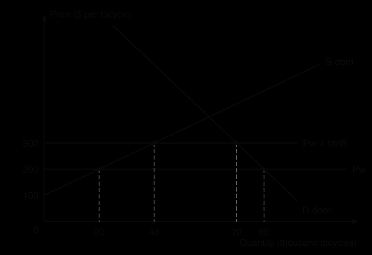
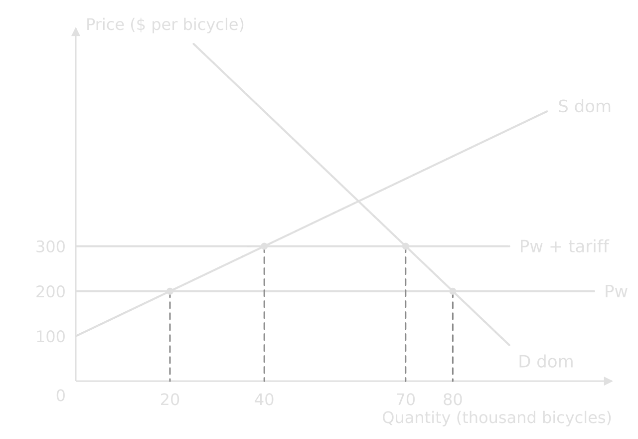
Tariff diagram for bicycles: domestic D and S, world price $200 and Pw + tariff $300. At $200 domestic supply is 20 thousand and demand 80 thousand; at $300 supply is 40 thousand and demand 70 thousand.Tariff diagram for bicycles: domestic D and S, world price $200 and Pw + tariff $300. At $200 domestic supply is 20 thousand and demand 80 thousand; at $300 supply is 40 thousand and demand 70 thousand.
Domestic demand and supply for bicycles with the world price $200 and the price after a $100 tariff, $300. Imports are the gap between domestic demand and supply at each price.

At the world price of $200, domestic firms supply 20 thousand bicycles and consumers buy 80 thousand, so imports are 80 − 20 = 60 thousand and import expenditure is $200 × 60 000 = $12 million. When the world price is above the domestic equilibrium, the same method gives exports (domestic supply − domestic demand) and export revenue (world price × exports).

Tariffs, quotas and production subsidies (HL only)

HL only

HL students calculate the effects of tariffs, quotas and production subsidies on consumers, domestic producers, foreign producers and the government from a diagram.

Worked example

The government imposes a tariff of $100 per bicycle (see the diagram). Calculate: (a) the change in imports and in import expenditure; (b) government tariff revenue; (c) the change in domestic producers’ revenue; (d) the welfare loss.

Show the solution
Tariff diagram with areas between $200 and $300: a, producer surplus gain left of supply; b, hatched triangle from 20 to 40 thousand; c, tariff revenue rectangle from 40 to 70 thousand; d, hatched triangle from 70 to 80 thousand.Tariff diagram with areas between $200 and $300: a, producer surplus gain left of supply; b, hatched triangle from 20 to 40 thousand; c, tariff revenue rectangle from 40 to 70 thousand; d, hatched triangle from 70 to 80 thousand.
a is the gain to domestic producers, c the tariff revenue, and the hatched triangles b and d the welfare loss.

(a) At $300, domestic supply is 40 thousand and demand 70 thousand, so imports fall from 60 to 30 thousand. Import expenditure (paid to foreign producers at the world price) falls from $12 million to $200 × 30 000 = $6 million.

(b) Tariff revenue (area c) = tariff × imports = $100 × 30 000 = $3 million.

(c) Domestic producers’ revenue rises from $200 × 20 000 = $4 million to $300 × 40 000 = $12 million: +$8 million.

(d) Welfare loss = b + d. Triangle b (inefficient domestic production) = ½ × (40 000 − 20 000) × 100 = $1 million. Triangle d (lost consumption) = ½ × (80 000 − 70 000) × 100 = $0.5 million. Total $1.5 million.

A quota of 30 thousand bicycles has the same effect on price and quantities, because the domestic price rises until imports equal 30 thousand (at $300). The difference is area c: instead of tariff revenue for the government, it becomes quota rent for the foreign exporters or licence holders, (300 − 200) × 30 000 = $3 million.

A production subsidy of $100 per bicycle to domestic firms leaves the price at $200 but lets producers receive $300, so domestic supply rises to 40 thousand while consumers still buy 80 thousand. Imports fall to 40 thousand (import expenditure $8 million), the subsidy costs the government $100 × 40 000 = $4 million, producers’ revenue including the subsidy rises to $12 million, and the welfare loss is triangle b only ($1 million), since consumers are unaffected.

Common mistake

Calculating tariff revenue as the tariff × the original imports (60 thousand). The tariff is paid only on the imports that still arrive after it, 30 thousand.

Opportunity cost and comparative advantage (HL only)

HL only

HL students calculate opportunity costs from data to identify comparative advantage, and draw linear PPCs to show it.

A country has comparative advantage in a good if it can produce it at a lower opportunity cost than another country. The opportunity cost of one unit of a good is the amount of the other good given up.

opportunity cost of 1 unit of X=units of Y given upunits of X gainedopportunity cost of 1 unit of X=units of X gainedunits of Y given up​

Worked example

Using all their resources, Alba can produce 200 thousand tonnes of rice or 100 thousand metres of cloth; Bora can produce 80 thousand tonnes of rice or 80 thousand metres of cloth. Calculate the opportunity costs, and identify which country has the absolute and the comparative advantage in each good.

Show the solution

Step 1: opportunity cost of 1 metre of cloth. Alba gives up 200 ÷ 100 = 2 tonnes of rice; Bora gives up 80 ÷ 80 = 1 tonne.

Step 2: opportunity cost of 1 tonne of rice. Alba gives up 100 ÷ 200 = 0.5 metres of cloth; Bora gives up 80 ÷ 80 = 1 metre.

Linear PPCs: rice (thousand tonnes) against cloth (thousand metres). Alba's runs from 200 rice to 100 cloth; Bora's from 80 rice to 80 cloth, so Alba's is steeper.Linear PPCs: rice (thousand tonnes) against cloth (thousand metres). Alba's runs from 200 rice to 100 cloth; Bora's from 80 rice to 80 cloth, so Alba's is steeper.
The slope of each linear PPC is the opportunity cost of cloth in terms of rice. Alba’s steeper PPC means cloth costs Alba more rice.

Step 3: identify. Alba has the absolute advantage in both goods (it can produce more of each). Alba has the comparative advantage in rice (0.5 < 1) and Bora in cloth (1 < 2). Both gain if Alba specialises in rice and Bora in cloth and they trade at a rate between 1 and 2 tonnes of rice per metre of cloth.

Common mistake

Identifying comparative advantage from the larger output. Alba produces more of both goods, but comparative advantage depends only on the opportunity cost ratios, so Bora still has the comparative advantage in cloth.

The Marshall–Lerner condition (HL only)

HL only

HL students apply the Marshall–Lerner condition to judge whether a depreciation improves the current account.

A depreciation improves the current account only if the sum of the price elasticities of demand for exports and imports (as absolute values) is greater than 1. If PED for exports is 0.4 and for imports 0.5, the sum is 0.9: below 1, so the current account worsens at first, as the J-curve shows. If, after two years, the elasticities rise to 0.8 and 0.7, the sum is 1.5 and the depreciation improves the current account.

Traps that cost marks in every unit

The same few errors account for most of the marks lost on calculations. The table lists them with the fix for each.

Trap

Fix

Wrong base for a percentage change

Divide by the old (starting) value.

Elasticity upside down

Quantity on top: %ΔQ ÷ %ΔP (or %ΔY).

Sign dropped

Keep minus signs on YED, growth, the current account and exchange rate changes.

Units missing or wrong scale

Read axis and table headings; write $ thousand, $ billion, %, tonnes.

Percent vs percentage points

A difference between two rates is in percentage points.

Rounding too early

Keep full figures until the final answer; round to 2 decimal places.

Nominal instead of real

Deflate before calculating growth or per capita living standards.

Old quantity in a revenue calculation

Use the quantity after the tax, subsidy or tariff.

MC = TC ÷ Q

MC = ΔTC ÷ ΔQ; TC ÷ Q is AC.

Multiplier with only MPS

Add every leakage given: MPS + MPT + MPM.

A calculation answer earns full marks only with valid working, the correct number and the correct unit. Writing the formula and the substitution makes the method mark safe even when the arithmetic goes wrong.

Add to your notes: a single page with every formula in the course, grouped by unit, each with its unit and one trap. Rewrite it from memory once a week before the exams.

Practice set

Try each item before opening the answer. Every answer shows the working that would earn full marks.

Worked example

(Paper 2 style) (a) A country’s CPI rises from 124.0 to 130.2. Calculate the inflation rate. [2] (b) Nominal GDP is $85 billion and the GDP deflator is 125. Calculate real GDP. [2] (c) The price of a good rises by 5% and quantity demanded falls by 2%. Calculate the PED and state whether demand is elastic or inelastic. [2]

Show the solution

(a) (130.2 − 124.0) ÷ 124.0 × 100 = 5%.

(b) 85 ÷ 125 × 100 = $68 billion.

(c) PED = −2 ÷ 5 = −0.4: price inelastic, since 0.4 < 1.

Tip

After each answer, ask whether the number makes sense. A real GDP above nominal GDP when the deflator is above 100, a negative PES, or an unemployment rate above 100% signals an error before any marks are lost.

Worked example

(Paper 3 style) (a) MPC is 0.8 in a closed economy with no taxes. Calculate the change in real GDP after a $3 billion rise in investment. [2] (b) At a world price of $5, domestic demand is 900 units and domestic supply 300 units. Calculate import expenditure. [2] (c) A household earns $30 000 and pays $4 500 in income tax. Calculate its average tax rate. [1]

Show the solution

(a) k = 1 ÷ (1 − 0.8) = 5; ΔY = 5 × 3 = $15 billion.

(b) Imports = 900 − 300 = 600 units; import expenditure = 5 × 600 = $3 000.

(c) 4 500 ÷ 30 000 × 100 = 15%.

Summary

  • Every calculation is marked for method and answer: write the formula, the substitution and the answer with its unit.

  • Percentage change divides by the old value; elasticities put the percentage change in quantity on top.

  • Macro calculations use real values for growth and living standards, the labour force for unemployment, and weighted baskets for inflation.

  • HL market calculations are rectangles (revenue, spending, tax, subsidy cost) and triangles (surplus, welfare loss) on a diagram.

  • HL macro calculations include the multiplier with every leakage, tax bands applied band by band, and Lorenz curves from cumulative shares.

  • HL trade calculations read imports and prices off the diagram; comparative advantage comes from opportunity cost, not output.

Self-check

  • To do:

    I can calculate a percentage change and tell percentages from percentage points.

  • To do:

    I can calculate PED, YED and PES, and use them to find a missing change in quantity or total revenue.

  • To do:

    I can calculate nominal and real GDP and GNI, per capita values, growth, unemployment, inflation and real interest rates.

  • To do:

    I can calculate the BoP balances, a price in another currency and a currency’s percentage change.

  • To do:

    I can calculate surplus, tax, subsidy and price control effects and welfare loss from a diagram (HL).

  • To do:

    I can calculate MR, MC, AR, AC and profit from a table and find the profit-maximising output (HL).

  • To do:

    I can calculate a weighted price index, tax paid and average tax rates, and construct a Lorenz curve (HL).

  • To do:

    I can calculate the multiplier, opportunity costs and the effects of tariffs, quotas and subsidies (HL).

Keep your place

In Augment the notes remember where you stopped and which pages you have finished.

Open in Augment

More IB Economics notes

  • Paper 2: data responseThe page before this.
  • Paper 3: policy paperThe next page. HL only.
  • Economics assessmentEach Economics paper, the internal assessment and grade boundaries.
  • IB EconomicsThe Economics syllabus, how it is assessed and every notes page.

Carry on with Economics in Augment

With a free account, Augment remembers where you stopped in the notes and which questions you have marked.

Start free