Data analysis

How to record raw data with uncertainties, propagate them through calculations, and draw and use graphs: tangents, gradients with uncertainties, calibration curves, extrapolation and linearized plots.

IB Chemistry
Internal assessment
SL and HL

23 min readLast reviewed 14 Oct 2026

The Data analysis criterion assesses how the raw data are recorded, how they are processed into the quantities that answer the research question, and how they are presented. Uncertainties run through all three. A top-level analysis is clear, so a reader can follow every step, and precise, so every number has a unit, an appropriate number of decimal places or significant figures, and an uncertainty. The processing is correct and relevant to the question.

Analysis turns a table of readings into evidence. The usual route in chemistry is raw data, then means and their uncertainties, then a derived quantity (a rate, a concentration, an enthalpy change) with a propagated uncertainty, then a graph that tests the predicted relationship, and finally a gradient, intercept or interpolated value that can be compared with theory or a literature value. Each step is shown once, with a sample calculation, so that a moderator can check it.

What the criterion rewards

Strand	1–2	3–4	5–6
Communication of recording and processing	Neither clear nor precise	Clear or precise	Clear and precise
Uncertainties	Limited evidence of consideration	Considered, with some significant omissions or inaccuracies	Considered appropriately
Processing relevant to the question	Some, with major omissions, inaccuracies or inconsistencies	Carried out, with some significant omissions, inaccuracies or inconsistencies	Carried out appropriately and accurately

"Clear" means the method of processing can be understood easily: labelled tables, one sample of each calculation, graphs that are easy to read. "Precise" means following the conventions: units, decimal places consistent with the instrument, significant figures matched to the uncertainty, titled and annotated graphs and tables. A beautifully presented analysis with every value given to eight significant figures is clear but not precise.

The clarifications also distinguish two kinds of fault. A major omission, inaccuracy or inconsistency prevents a valid conclusion from being drawn at all, for example calculating initial rates from the wrong part of the curve. A significant one still allows a conclusion, but limits its validity or detail, for example leaving out the uncertainty of the gradient.

Recording raw data

Raw data go into a table as they are taken. A raw data table that follows the conventions earns the "precise" strand almost automatically.

Each column heading gives the quantity, its unit and its uncertainty, for example "Volume of $H_{2}$ / ${cm}^{3}$ ( $\pm 0.5$ )". Units and uncertainties go in the heading, not after every number.
Every value in a column has the same number of decimal places, matching the resolution of the instrument. A burette reading is recorded as $23.40$ , not $23.4$ ; a balance to two decimal places gives $1.00$ g, not $1$ g.
The independent variable is in the first column, and repeats are in separate columns, side by side.
The table has a title that says what was measured and under what conditions.

Time / s (±0.5)	Volume of $H_{2}$ / ${cm}^{3}$ ( $\pm 0.5$ ), run 1	Run 2	Run 3	Mean volume / ${cm}^{3}$
10	10.0	9.5	10.0	9.8
20	17.5	17.0	17.0	17.2
30	23.0	22.5	23.0	22.8
40	27.5	27.0	27.0	27.2
60	33.0	32.5	33.0	32.8
120	39.5	39.0	39.5	39.3

Sample data: hydrogen collected from 4.0 cm of magnesium ribbon in 50.0 cm³ of 0.75 mol dm⁻³ hydrochloric acid at 25.0 °C (selected rows).

The means are given to one decimal place, the same as the readings. Giving them to three decimal places would claim a precision the data do not have. The half-range of each set of repeats (at most $0.25 {cm}^{3}$ ) is smaller than the syringe uncertainty, so $\pm 0.5 {cm}^{3}$ is the uncertainty quoted for each mean.

Qualitative observations

Qualitative data are recorded alongside the numbers, in a column or a short list. In the magnesium investigation, useful observations include bubbles clinging to the ribbon and lifting it to the surface, a grey film on the metal before cleaning, the solution warming slightly, and the time at which the ribbon disappeared. Each of these may later explain a feature of the data or a weakness of the method, and the evaluation is far stronger when it can point to them.

The uncertainty of a single reading

Every reading carries an absolute uncertainty, written with the same unit as the reading: $27.0 \pm 0.5 {cm}^{3}$ . For a scale read by eye, the uncertainty is usually half the smallest division (a gas syringe marked every $1 {cm}^{3}$ gives $\pm 0.5 {cm}^{3}$ ). For a digital display, it is one unit of the last digit (a balance showing $1.00$ g gives $\pm 0.01$ g). For glassware such as pipettes and volumetric flasks, the tolerance printed on the glass is used.

Many chemistry measurements are differences between two readings: a titre is a final burette reading minus an initial one, a temperature change is a final temperature minus an initial one, and a mass of solid used is a mass before minus a mass after. Each of the two readings carries its own uncertainty, so the difference carries both. A burette titre therefore has an uncertainty of $\pm 0.10 {cm}^{3}$ , not $\pm 0.05 {cm}^{3}$ .

The percentage uncertainty shows how much a measurement matters. A titre of $23.45 \pm 0.10 {cm}^{3}$ has a percentage uncertainty of $0.43 %$ ; a temperature rise of $9.6 \pm 0.2$ K has $2.1 %$ . The temperature rise dominates the uncertainty of any calculation that uses both, which tells the student where improvement matters most.

The uncertainty from repeated readings

Repeating a measurement shows how much it varies because of random errors: small, unpredictable differences in judging the moment a cross disappears, in how quickly a bung is inserted, in the exact surface of a piece of magnesium. The mean of the repeats is the best estimate of the value, and a simple, widely accepted estimate of its random uncertainty is half the range:

uncertainty of the mean \approx \pm \frac{largest value - smallest value}{2}

For three initial rates of $1.05$ , $1.12$ and $1.19 {cm}^{3} s^{- 1}$ , the mean is $1.12 {cm}^{3} s^{- 1}$ and the uncertainty is $\pm (1.19 - 1.05) / 2 = \pm 0.07 {cm}^{3} s^{- 1}$ . When the half-range is smaller than the uncertainty of a single reading (for example, three identical readings), the instrument uncertainty is used instead, because the repeats cannot be more certain than the instrument that made them.

Outliers

An outlier is a value that does not fit the pattern of the other repeats or the trend of the graph. It is identified by inspection and removed only with a reason, which is stated in the report: a rough first titre, a run where the bung was inserted late, a reading taken after the syringe plunger stuck. Values are never removed just because they spoil a trend. If there is no reason, the value stays in, and its effect is discussed.

Titration has its own convention for this. A rough titre is taken first and excluded. Accurate titres are then repeated until at least two are concordant, agreeing within $0.10 {cm}^{3}$ , and only the concordant titres are averaged. For titres of $23.95$ (rough), $23.45$ , $23.40$ and $23.50 {cm}^{3}$ , the mean of the concordant titres is $23.45 {cm}^{3}$ .

Significant figures and decimal places

Uncertainties are given to one significant figure (occasionally two when the first digit is 1), and the value is then rounded to the same decimal place as its uncertainty. A calculated concentration of $0.093803 {mol dm}^{- 3}$ with an uncertainty of $0.000704$ is written $0.0938 \pm 0.0007 {mol dm}^{- 3}$ . Intermediate values are kept unrounded in the calculation and rounded only at the end.

Processing data

Propagating uncertainties

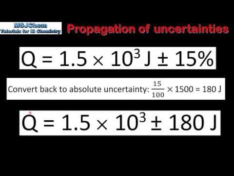
When measured values are combined in a calculation, their uncertainties combine too, a process called the propagation of uncertainties. The data booklet gives the rules used in IB Chemistry. For a sum or difference, the absolute uncertainties add; for a product or quotient, the fractional (or percentage) uncertainties add.

\begin{aligned} y & = a \pm b & Δ y & = Δ a + Δ b \\ y & = \frac{a b}{c} & \frac{Δ y}{y} & = \frac{Δ a}{a} + \frac{Δ b}{b} + \frac{Δ c}{c} \end{aligned}

Pure numbers and constants, such as the 1000 that converts ${cm}^{3}$ to ${dm}^{3}$ , the 2 in a mole ratio or the specific heat capacity of water taken from the data booklet, add no uncertainty. Adding uncertainties in this way gives the largest likely uncertainty, which is a cautious estimate.

A student titrates $25.00 {cm}^{3}$ of sodium hydroxide solution, measured with a pipette ( $\pm 0.03 {cm}^{3}$ ), with $0.1000 \pm 0.0002 {mol dm}^{- 3}$ hydrochloric acid. The mean concordant titre is $23.45 \pm 0.10 {cm}^{3}$ . Calculate the concentration of the sodium hydroxide with its absolute uncertainty.

Show the solution

Concentration. The acid and base react 1 : 1, so $C_{N a O H} V_{N a O H} = C_{H C l} V_{H C l}$ :

C_{N a O H} = \frac{0.1000 \times 23.45}{25.00} = 0.09380 {mol dm}^{- 3}

Percentage uncertainties of the three measured quantities:

\begin{aligned} titre: & \frac{0.10}{23.45} \times 100 = 0.43 % \\ pipette: & \frac{0.03}{25.00} \times 100 = 0.12 % \\ acid concentration: & \frac{0.0002}{0.1000} \times 100 = 0.20 % \end{aligned}

Add them (a product and a quotient): $0.43 + 0.12 + 0.20 = 0.75 %$ .

Absolute uncertainty: $0.0075 \times 0.09380 = 0.0007 {mol dm}^{- 3}$ , so $C_{N a O H} = 0.0938 \pm 0.0007 {mol dm}^{- 3}$ .

The titre contributes more than half of the total, so more precise end-point detection would improve the result most.

A calorimetry calculation combines a temperature change, a mass and an amount in the same way. The extrapolated temperature rise is usually the largest source of uncertainty.

When excess zinc powder is added to $50.00 \pm 0.10 {cm}^{3}$ of $0.200 \pm 0.001 {mol dm}^{- 3}$ copper(II) sulfate, the extrapolated temperature rise is $9.6 \pm 0.2$ K. Calculate the enthalpy change of the reaction with its uncertainty. Assume the solution has a density of $1.00 {g cm}^{- 3}$ and $c = 4.18 {J g}^{- 1} K^{- 1}$ .

Show the solution

Heat released: $Q = m c Δ T = 50.00 \times 4.18 \times 9.6 = 2006 J$ .

Amount of copper(II) sulfate (the limiting reactant): $n = 0.200 \times 0.05000 = 0.01000 mol$ .

Enthalpy change (exothermic, so negative):

Δ H = - \frac{2006}{0.01000} = - 2.006 \times 10^{5} {J mol}^{- 1} = - 200.6 {kJ mol}^{- 1}

Uncertainty. The volume appears in both $m$ (as $ρ V$ ) and $n$ (as $C V$ ), so it cancels: $Δ H = - ρ c Δ T / C$ . Only $Δ T$ and $C$ contribute:

\frac{0.2}{9.6} \times 100 + \frac{0.001}{0.200} \times 100 = 2.1 % + 0.5 % = 2.6 %

$0.026 \times 200.6 = 5 {kJ mol}^{- 1}$ , so $Δ H = - 201 \pm 5 {kJ mol}^{- 1}$ .

Mike Sugiyama Jones (MSJ Chem): propagation of uncertainties. Made for the previous course, but the methods are the same.

Showing the processing

Each type of calculation is shown once, in full, as a sample calculation with the numbers substituted, units included and the result rounded correctly. The results of repeating it for every row then go into a table of processed data, which has the same conventions as a raw data table: quantity, unit and uncertainty in each heading, consistent decimal places. A spreadsheet can do the arithmetic, but the report must still show one worked example of each formula so that the moderator can check it.

$[H C l]$ / ${mol dm}^{- 3}$ ( $\pm 0.005$ )	Initial rate, runs 1–3 / ${cm}^{3} s^{- 1}$	Mean initial rate / ${cm}^{3} s^{- 1}$
0.250	0.36, 0.38, 0.41	$0.38 \pm 0.03$
0.500	0.69, 0.73, 0.78	$0.73 \pm 0.05$
0.750	1.05, 1.12, 1.19	$1.12 \pm 0.07$
1.000	1.42, 1.50, 1.59	$1.50 \pm 0.09$
1.250	1.72, 1.83, 1.95	$1.83 \pm 0.12$

Sample processed data: initial rates from tangents at t = 0, with uncertainties from half the range of three runs.

Graphs

Drawing a good graph

A graph of the processed data is the centre of most chemistry analyses: it tests the predicted relationship, shows the scatter of the data and gives a gradient or intercept to compare with theory. A graph that communicates clearly and precisely has:

a title that states the relationship shown;
the independent variable on the x-axis and the dependent (or processed) variable on the y-axis, each labelled with the quantity and its unit, as in " $[H C l]$ / ${mol dm}^{- 3}$ ";
scales that use most of the available area and are easy to read (steps of 1, 2 or 5 units), starting from zero only when the origin is meaningful;
each point plotted precisely, with an error bar showing its uncertainty in y (and in x where it is visible at the scale used);
a single line or smooth curve of best fit, never a dot-to-dot line joining the points.

Error bars show at a glance whether the scatter is consistent with the uncertainties: if a straight line of best fit passes through every error bar, the data are consistent with a linear relationship. Spreadsheet software draws the line by least squares and reports its equation and the coefficient of determination, $R^{2}$ .

$R^{2}$ is useful but limited. A value of $0.999$ shows that points lie very close to the line; it does not show that a straight line is the right model, that the line should pass through the origin, or that the data are accurate. Data with a gentle curve can still give $R^{2} > 0.99$ with a straight line, which is why the pattern of points either side of the line (the residuals) is worth checking by eye.

Rates from graphs: tangents

The rate of a reaction at any moment is the gradient of a concentration–time (or volume–time) curve at that moment. Because the curve flattens as reactants are used up, the gradient changes continuously, and the rate at an instant is found by drawing a tangent: a straight line that touches the curve at that point without crossing it. The initial rate is the gradient of the tangent at $t = 0$ , when the concentrations are known exactly.

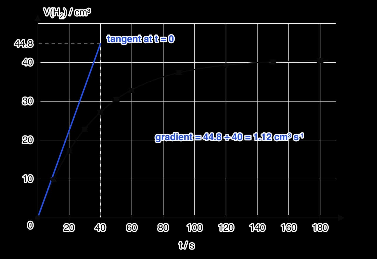
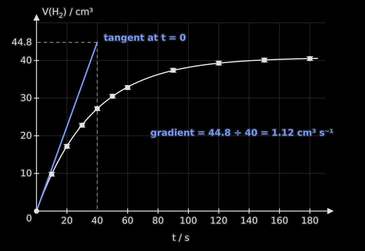
Graph of the volume of hydrogen in cm³ against time in seconds for 0.75 mol dm⁻³ acid. Mean points with error bars of ±0.5 cm³ lie on a smooth curve that rises steeply then levels off near 40.8 cm³. — Sample data; the error bars show the syringe uncertainty (±0.5 cm³), larger than the half-range of the repeats. The initial rate is the gradient of the tangent (blue) drawn at t = 0. A long tangent, read at a point far from the origin, gives the most precise gradient.

The tangent for the $0.75 {mol dm}^{- 3}$ run rises $44.8 {cm}^{3}$ in $40$ s, so the initial rate is $44.8 \div 40 = 1.12 {cm}^{3} s^{- 1}$ . Drawing tangents by eye is subjective. More reproducible alternatives are to fit a curve to the data in a spreadsheet and calculate its gradient at $t = 0$ , or to use the average rate over the first few seconds, when the curve is still nearly straight (here, $9.8 {cm}^{3}$ in the first 10 s, $0.98 {cm}^{3} s^{- 1}$ , already about 12 % below the tangent value). Whichever method is used must be the same for every run, and its limitation belongs in the evaluation.

Gradients and their uncertainty

When the graph is a straight line, its gradient (and sometimes its intercept) is usually the processed result. The uncertainty of the gradient comes from the error bars: draw the steepest and the shallowest straight lines that still pass through every error bar. Their gradients give the range within which the true gradient lies.

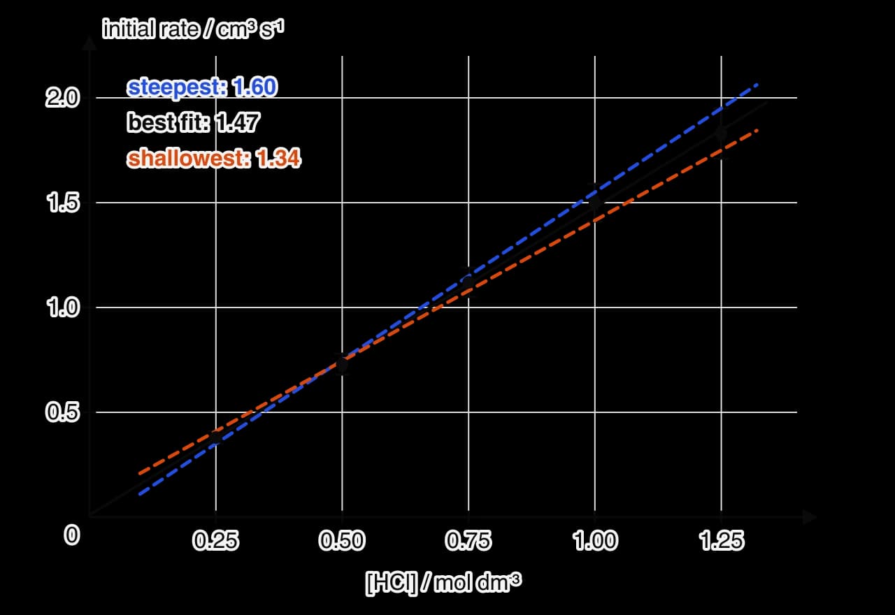
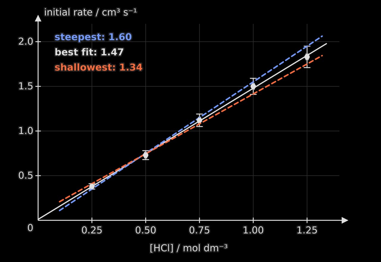
uncertainty in gradient = \pm \frac{steepest gradient - shallowest gradient}{2}

Graph of initial rate in cm³ s⁻¹ against hydrochloric acid concentration from 0 to 1.4 mol dm⁻³. Five points with vertical error bars growing from ±0.03 to ±0.12 lie close to a straight black best-fit line of gradient 1.47 that passes almost through the origin. — Sample data. The best-fit line (black) and the steepest and shallowest straight lines that pass through every error bar (blue and orange, dashed). Half the difference between their gradients, ±0.13, is the uncertainty in the gradient.

For the graph of initial rate against concentration, the best-fit gradient is $1.47 {cm}^{3} s^{- 1} {mol}^{- 1} {dm}^{3}$ , the steepest line has $1.60$ and the shallowest $1.34$ . The gradient is therefore $1.47 \pm 0.13 {cm}^{3} s^{- 1} {mol}^{- 1} {dm}^{3}$ , a percentage uncertainty of about $9 %$ . The intercept of the best-fit line, $0.01 {cm}^{3} s^{- 1}$ , lies between those of the steepest and shallowest lines ( $- 0.05$ and $+ 0.08$ ), so it is zero within uncertainty. A straight line through the origin means the initial rate is directly proportional to the concentration of the acid over this range.

Calibration curves and interpolation

Colorimetry measures absorbance, not concentration. To convert one into the other, a calibration curve is made from standard solutions of known concentration, prepared by diluting a stock solution with a burette or pipette and volumetric flasks. Over a suitable range, absorbance is directly proportional to concentration, so the standards fall on a straight line.

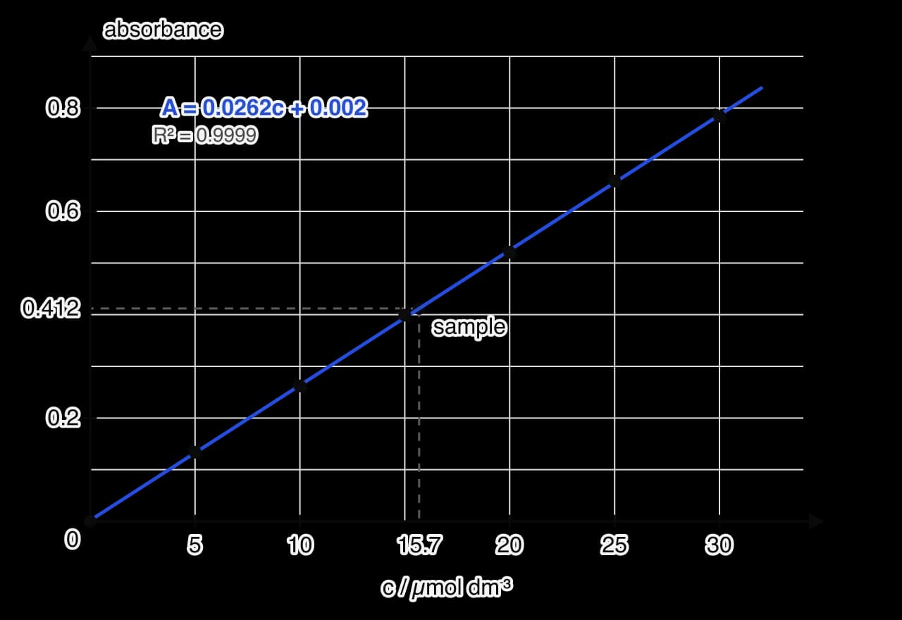
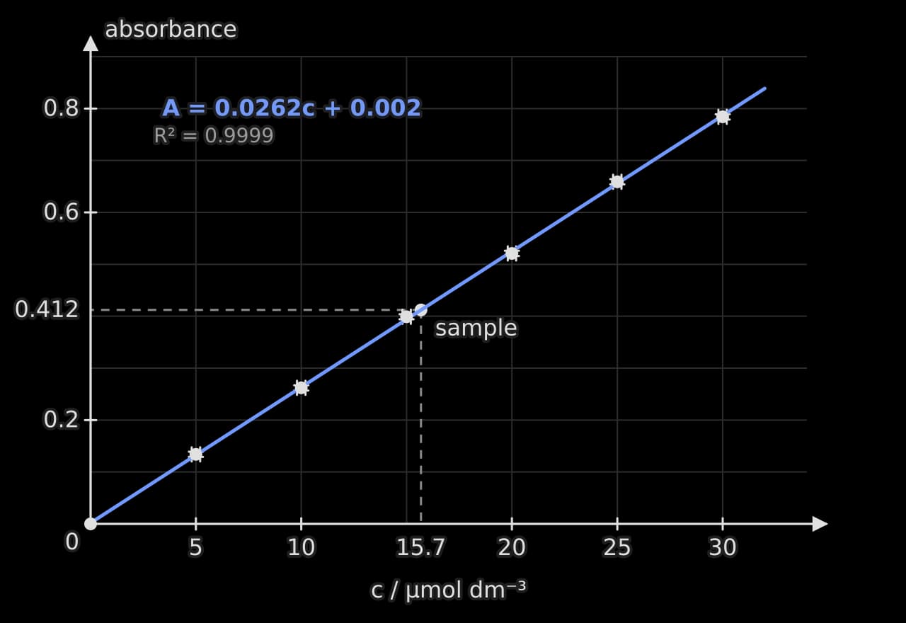
Calibration graph of absorbance against dye concentration from 0 to 34 µmol dm⁻³. Seven standards lie on a straight blue line through the origin, labelled A = 0.0262c + 0.002 with R² = 0.9999; error bars are very small. — Sample data. Standards of known concentration give a straight calibration line (blue). The concentration of the sample is read off by interpolation, inside the range of the standards.

A sports drink, diluted so that its absorbance falls within the range of the standards, gives an absorbance of $0.412$ . Reading across to the line and down to the axis, or rearranging the line’s equation, gives the concentration of the dye in the diluted drink: $c = (0.412 - 0.002) \div 0.0262 = 15.7 μ {mol dm}^{- 3}$ . Reading a value inside the range of the data is interpolation and is reliable; reading beyond it is extrapolation and assumes the relationship continues, which for absorbance often fails at high concentrations.

Extrapolation in calorimetry

In a polystyrene-cup experiment, the reaction takes time to finish while heat is already escaping, so the highest temperature recorded is lower than the temperature the mixture would have reached with no heat loss. Plotting temperature against time and extrapolating the cooling line back to the moment of mixing corrects for the heat lost during the reaction.

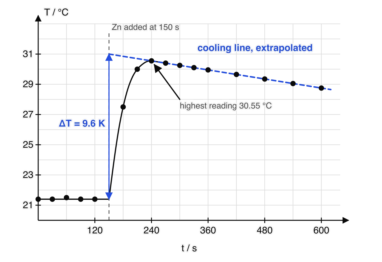
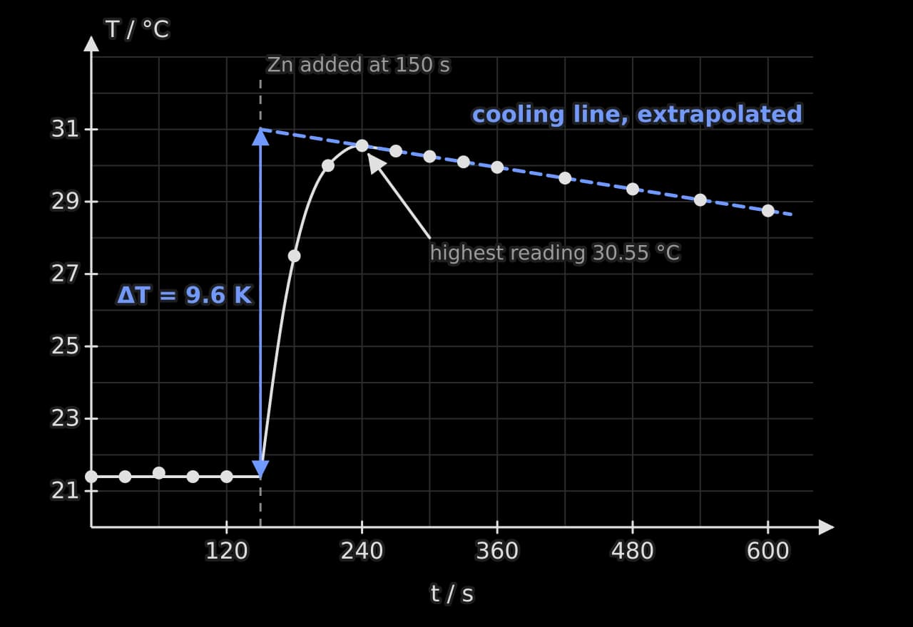
Graph of temperature in °C against time in seconds. The temperature is steady at 21.4 °C until zinc is added at 150 s, marked by a dashed vertical line. It then rises to a highest reading of 30.55 °C at 240 s and falls slowly in a straight line. — Sample data for 0.200 mol dm⁻³ copper(II) sulfate with excess zinc. Extrapolating the cooling line (blue) back to the time of mixing estimates the temperature that would have been reached with no heat loss, giving ΔT = 9.6 K rather than the 9.15 K between the starting and highest readings.

The starting temperature, $21.4$ °C, is the steady value before mixing. The cooling line extrapolated back to $150$ s reaches $31.0$ °C, so $Δ T = 9.6$ K. Using the highest reading instead would give $9.15$ K, a result about 5 % too small. Extrapolation reduces the systematic error from heat loss but cannot remove it entirely, because it assumes the rate of heat loss was the same during the reaction as afterwards.

Exponents and linearized graphs (HL)

Uncertainty of a power

When a measured quantity is raised to a power, its fractional uncertainty is multiplied by the size of the power (data booklet):

y = a^{n} \frac{Δ y}{y} = ∣ n \frac{Δ a}{a} ∣

Squaring a concentration of $0.200 \pm 0.004 {mol dm}^{- 3}$ (2 %) in a second-order rate equation gives a 4 % uncertainty in $[A]^{2}$ . A reciprocal is a power of $- 1$ , so a reaction time of $14 \pm 1$ s (7 %) gives a rate, proportional to $1 / t$ , with the same 7 % uncertainty. The absolute value in the rule means that a negative power still increases the uncertainty; it never cancels it.

Linearizing the Arrhenius equation

Many relationships in chemistry are not straight lines, and a curve is hard to test or extract a constant from. Rearranging the equation so that a graph of two processed quantities should be straight, called linearization, turns the constant into a gradient or intercept. The Arrhenius equation is the most common example:

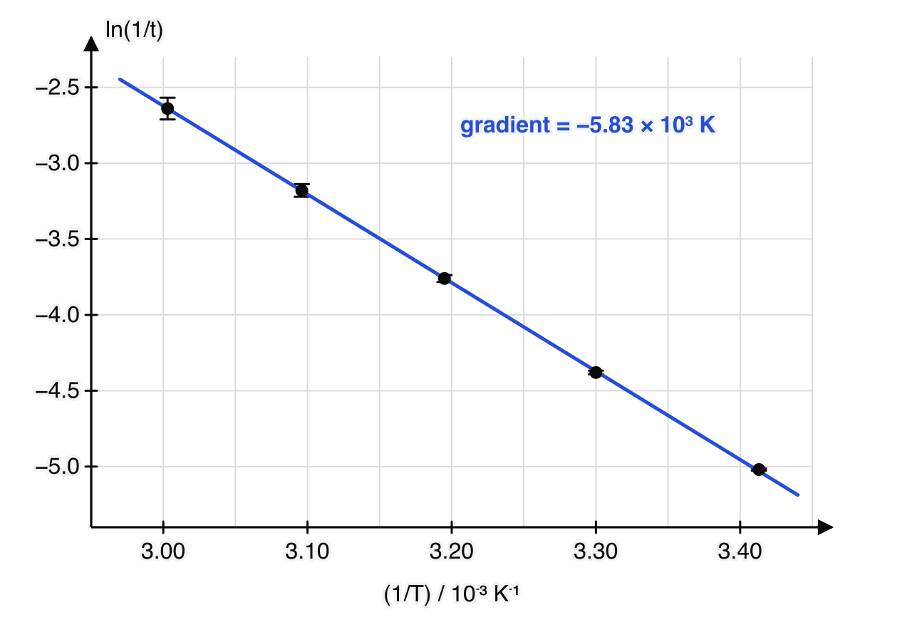
k = A e^{- E_{a} / R T} ⟹ \ln k = - \frac{E_{a}}{R} \cdot \frac{1}{T} + \ln A

A graph of $\ln k$ against $1 / T$ is a straight line with gradient $- E_{a} / R$ . In a "disappearing cross" investigation of the reaction between sodium thiosulfate and hydrochloric acid, the concentrations are the same at every temperature, so the rate constant is proportional to the rate, and the rate to $1 / t$ , where $t$ is the time for the cross to disappear. A graph of $\ln (1 / t)$ against $1 / T$ therefore has the same gradient as the Arrhenius plot.

θ / °C (±0.5)	T / K	t / s (±1)	$(1 / T)$ / $10^{- 3} K^{- 1}$	$\ln (1 / t)$
20.0	293	152	3.413	$- 5.02 \pm 0.01$
30.0	303	80	3.300	$- 4.38 \pm 0.01$
40.0	313	43	3.195	$- 3.76 \pm 0.02$
50.0	323	24	3.096	$- 3.18 \pm 0.04$
60.0	333	14	3.003	$- 2.64 \pm 0.07$

Sample data: mean times for the cross to disappear, with ln(1/t) and its uncertainty from the timing uncertainty.

Graph of ln(1/t) against 1/T in units of 10⁻³ K⁻¹, from 2.95 to 3.45. Five points from 20 °C to 60 °C fall on a straight blue line sloping downwards to the right, with gradient −5.83 × 10³ K. Error bars grow from very small at the lowest temperature to ±0.07 at the highest. — Sample data. Because the rate is proportional to 1/t, a graph of ln(1/t) against 1/T has the same gradient as ln k against 1/T, −Ea/R. The error bars are largest at high temperature, where the reaction time is shortest.

The best-fit line of the graph of $\ln (1 / t)$ against $1 / T$ has a gradient of $- 5.83 \times 10^{3}$ K. The steepest and shallowest lines through all the error bars have gradients of $- 5.85 \times 10^{3}$ K and $- 5.67 \times 10^{3}$ K. Determine the activation energy with its uncertainty.

Show the solution

Activation energy from gradient $= - E_{a} / R$ , with $R = 8.31 {J K}^{- 1} {mol}^{- 1}$ :

E_{a} = - (gradient) \times R = 5.83 \times 10^{3} \times 8.31 = 4.84 \times 10^{4} {J mol}^{- 1} = 48.4 {kJ mol}^{- 1}

Uncertainty of the gradient: $\pm (5.85 - 5.67) \times 10^{3} / 2 = \pm 0.09 \times 10^{3}$ K, about $1.5 %$ .

Uncertainty of $E_{a}$ : $R$ is a constant, so the percentage uncertainty is the same, $0.015 \times 48.4 = 0.7 {kJ mol}^{- 1}$ . The result is $E_{a} = 48.4 \pm 0.7 {kJ mol}^{- 1}$ .

This uncertainty reflects only the $\pm 1$ s timing uncertainty used for the error bars. Where the repeats spread more widely (for example times of 12, 14 and 16 s at 60 °C, a half-range of $\pm 2$ s), the error bars are larger, the steepest and shallowest lines move further apart and the uncertainty in $E_{a}$ grows.

Error bars on a logarithmic axis

For a natural logarithm, a small absolute uncertainty in $\ln x$ equals the fractional uncertainty in $x$ : $Δ (\ln x) \approx Δ x / x$ . A reaction time of $14 \pm 1$ s therefore gives $\ln (1 / t)$ an uncertainty of about $\pm 1 / 14 = \pm 0.07$ . This is why the error bars in the Arrhenius plot grow at high temperature: the absolute timing uncertainty stays at about 1 s while the times themselves get shorter. Strictly the temperature uncertainty also gives a horizontal error bar, but $\pm 0.5$ K changes $1 / T$ by less than 0.2 %, too small to show at this scale.

Applying the ideas

A titre with its uncertainty

Amount of acid from a concentration

Reading a gradient

On a graph of initial rate against concentration, a student finds the best-fit gradient is $2.15 {cm}^{3} s^{- 1} {mol}^{- 1} {dm}^{3}$ , the steepest line $2.41$ and the shallowest $1.95$ , with an intercept of $- 0.21 {cm}^{3} s^{- 1}$ that lies outside the range of the steepest and shallowest intercepts. State the gradient with its uncertainty, and comment on the intercept.

Show the answer

Gradient: $\pm (2.41 - 1.95) / 2 = \pm 0.23$ , so $2.2 \pm 0.2 {cm}^{3} s^{- 1} {mol}^{- 1} {dm}^{3}$ (the value is rounded to the same decimal place as its one-significant-figure uncertainty).

Intercept: a negative intercept that is not zero within uncertainty suggests a systematic error, for example a delay between adding the magnesium and starting the clock, or an oxide layer that slows the start of every run by a similar amount. It also means the rate is not simply proportional to concentration over the range measured.

Choosing between methods

Self-check

To do:
I can record raw data in a table with quantities, units and uncertainties in the headings and consistent decimal places.
To do:
I can record qualitative observations alongside quantitative data.
To do:
I can find the uncertainty of a single reading, of a difference between two readings and of the mean of repeats.
To do:
I can identify an outlier and justify excluding or keeping it, and average only concordant titres.
To do:
I can propagate uncertainties through sums, differences, products and quotients, and give results to an appropriate precision.
To do:
I can draw a graph with labelled axes, error bars and a line of best fit, and interpret R².
To do:
I can find an initial rate by drawing a tangent to a volume–time or concentration–time curve.
To do:
I can find a gradient and its uncertainty from the steepest and shallowest lines through the error bars, and interpret the intercept.
To do:
I can use a calibration curve to find a concentration by interpolation.
To do:
I can correct a calorimetry temperature change for heat loss by extrapolating a cooling line.
To do:
I can propagate uncertainties through powers and determine an activation energy from a linearized Arrhenius plot (HL).

Carry on with Chemistry in Augment

With a free account, Augment remembers where you stopped in the notes and which questions you have marked.

Start free