Data analysis

Data analysis is the second criterion of the scientific investigation. It assesses how the data are recorded, processed and presented, and how the uncertainty in them is handled. The aim of all three is to turn raw measurements into evidence that answers the research question.

The worked examples use one student's data from the sample investigation of the effect of temperature on catalase activity in potato tuber (Solanum tuberosum), whose method is set out in "Research design". The numbers are a student's sample results, chosen to show the processing steps, not published measurements.

What the criterion rewards

The descriptors look at the communication of recording and processing (whether it is clear and precise), the consideration of uncertainties, and whether the processing is relevant to the research question and carried out correctly.

Clear means that a reader can follow what was done: each table and graph is introduced in the text, every calculation type has a worked sample, and the reason for each processing step is given. Precise means that the conventions are followed: titles, units, uncertainties in column headings, consistent decimal places and correctly labelled axes. A major omission or inaccuracy stops a valid conclusion being drawn; a significant one still allows a conclusion but limits it.

Recording raw data

Raw data are recorded in a table at the time they are measured. The table holds every level of the independent variable and every repeat described in the method, so the reader can see that the planned data were collected. The independent variable goes in the first column; repeats of the dependent variable go in the columns after it.

Conventions for a data table

• A numbered, specific title: "Table 1: Volume of oxygen released by five potato discs in 60 s at seven temperatures".

• Each column heading gives the quantity, its unit and the uncertainty of the instrument: "Volume of O₂ / cm³ (±0.5 cm³)". Units go in the heading, not after every number.

• All values in a column have the same number of decimal places, matching the precision of the instrument. A gas syringe read to the nearest 0.5 cm³ gives values such as 8.0 and 8.5, never 8 and 8.50.

• Anomalous results are kept in the table and marked, not deleted.

• Qualitative observations (foaming, floating discs, colour changes) are recorded alongside, because they can help to explain the results.

The table of raw data is a student's sample results: Table 1, volume of oxygen collected in 60 s from 10.0 cm³ of 3% hydrogen peroxide with five potato discs. Each value is a direct reading from the gas syringe, so all have one decimal place. Because the collection time is 60 s, each volume is also the rate in cm³ min⁻¹.

Uncertainties

Every instrument has an uncertainty. For an analogue scale (a gas syringe, a thermometer, a measuring cylinder), it is usually taken as half the smallest division; for a digital instrument, it is the smallest digit it shows. The uncertainty of a timing by hand is larger than the stopwatch's resolution, because reaction time adds about 0.2–0.5 s. The uncertainty of each instrument is justified briefly in the report and shown in the column headings.

Percentage uncertainty

The size of an uncertainty matters only in comparison with the value measured. The percentage uncertainty compares them:

Variation between repeats

Instrument uncertainty is only one source of uncertainty. Repeats at the same temperature also differ from one another, because biological material varies (the discs differ slightly in catalase content and surface area) and because of small differences in technique. This variation is usually larger than the instrument uncertainty and is measured with the standard deviation or the range. Both kinds of uncertainty are considered in a strong report: the instrument uncertainty in the raw data, and the variation between repeats in the processed data and on the graph.

Processing the data

Processing means calculating from the raw data the quantities that answer the research question. Which calculations are relevant depends on the question, and each one is shown once as a sample calculation with its formula.

Means and standard deviations

The mean is the sum of the repeats divided by their number. The standard deviation measures how far the repeats spread around the mean; about 68% of values in a normal distribution lie within one standard deviation of the mean. A spreadsheet calculates both (AVERAGE and STDEV.S), but one sample calculation is shown by hand.

Table 2 holds the processed data, again a student's sample results. The standard deviation is largest at 50 °C, where catalase is partly denatured. Small differences between discs in how quickly they warm up, or in how much of their enzyme is denatured in the 60 s, have the biggest effect there, so the repeats spread more. Comments of this kind, linking the spread to the biology, are part of a clear analysis.

Percentage change and rates

Percentage change compares a change with the starting value, which allows results from samples of different sizes to be compared. It is calculated as (final − initial) ÷ initial × 100. Rates express the change in a quantity per unit time, read from a table (change ÷ time) or from the gradient of a graph.

Presenting data in graphs

A graph shows the relationship between the variables more clearly than a table. The type of graph depends on the data.

• Scatter graph with a line or curve of best fit: both variables continuous (temperature and rate). Means are plotted with error bars.

• Bar chart: categorical independent variable (species, site, type of sugar).

• Histogram: the frequency distribution of one continuous variable (leaf lengths in a sample).

• Box-and-whisker plot: compares the median and spread of several samples, especially when the data are skewed.

A good graph has a numbered, specific title, axes labelled with the quantity and unit ("Temperature / °C"), scales that use most of the grid, the independent variable on the x-axis, and a key or caption saying what the error bars show. A line or curve of best fit shows the trend; points are not joined dot to dot unless there is a reason to expect each point to be exact.

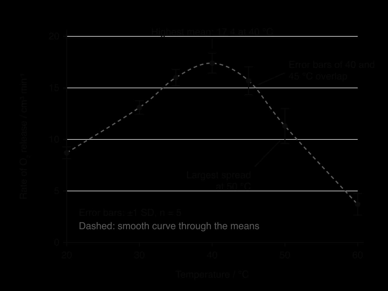
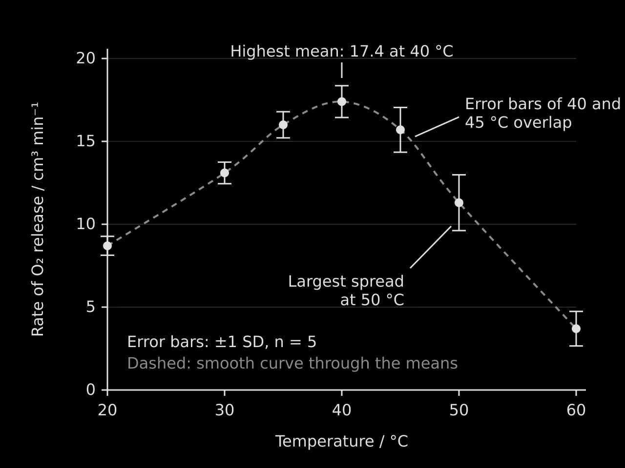
The graph of the sample results shows the shape expected from enzyme theory: a rise to a peak, then a steeper fall. Error bars add information that the means alone do not. Where the error bars of two means do not overlap (35 °C and 50 °C), the difference is probably real. Where they overlap (40 °C and 45 °C), the difference may be due to variation between discs, and a statistical test is used to decide.

Statistical tests

A statistical test is used to decide whether a difference or a relationship in the data is likely to be real or could have arisen by chance from the variation in the samples. Every test starts with a null hypothesis (there is no difference, or no relationship) and an alternative hypothesis. The test gives a value that is compared with a critical value, or a p-value. If p < 0.05, there is less than a 5% probability of a result this extreme if the null hypothesis were true, so the null hypothesis is rejected and the result has statistical significance.

Correlation in field data

In a correlation study, both variables are measured rather than one being set. The correlation coefficient (r) measures the strength and direction of a linear relationship, from −1 to +1, and the coefficient of determination (R²) gives the proportion of the variation in one variable that the line of best fit accounts for. A significant correlation does not show that one variable causes the other.

YouTube

Common mistakes and how to avoid them

• Inconsistent decimal places in a column, or more decimal places than the instrument can measure.

• Units or uncertainties missing from column headings and axis labels.

• Processing that does not answer the question, such as a bar chart of every raw value with no means or trend.

• No sample calculations, so the reader cannot check how a value was obtained.

• Anomalous results deleted without comment. An outlier may be excluded from a mean only with a stated reason (for example, the bung was found to be loose), and the raw value stays in the raw data table.

• Graphs of raw data only, with no means, error bars or trend line.