Practical techniques and biological drawing

A small number of laboratory and field techniques appear throughout the biology course: light microscopy, chromatography, colorimetry, sampling, karyotyping, molecular modelling and identification keys. Each is assessed in two ways. Paper 1B and Paper 2 questions ask you to describe the purpose of a technique, outline how it is carried out, process its results or evaluate it; the internal assessment asks you to use it well.

Each technique is set out with its purpose, the method, how results are processed and the most common sources of error, followed by the conventions for biological drawing, how variables are measured, and safety and ethics.

Light microscopy and temporary mounts

A light microscope magnifies specimens up to about ×400 with a school instrument (×1000 with oil immersion). Living cells can be viewed, but the specimen must be thin enough for light to pass through it, and most cell structures are colourless, so they are stained.

Preparing a temporary mount

A temporary mount is a specimen placed on a slide in a drop of liquid under a cover slip, for viewing on the same day.

1. Place a drop of water or stain in the centre of a clean slide.

2. Add a thin specimen, such as a single layer of onion epidermis peeled with forceps, or a leaf of the pondweed Elodea.

3. Lower a cover slip at an angle from one edge, using a mounted needle, so that air is pushed out and bubbles do not form.

4. Draw off excess liquid with filter paper; to stain an existing mount, add stain at one edge of the cover slip and draw it under with filter paper at the opposite edge.

Focusing and viewing

1. Start with the lowest-power objective lens and the stage at its lowest position.

2. Watching from the side, raise the stage with the coarse focus knob until the objective is close to the cover slip.

3. Looking through the eyepiece, lower the stage slowly with the coarse focus until the specimen is in focus, then sharpen it with the fine focus.

4. Move the area of interest to the centre, then turn to a higher-power objective and use only the fine focus.

5. Adjust the light with the diaphragm: less light often gives more contrast in unstained specimens.

Measuring with an eyepiece graticule

An eyepiece graticule is a small transparent scale fitted inside the eyepiece. It appears on top of the specimen at every magnification, but its divisions (eyepiece units) have no fixed size: the length of one eyepiece unit on the specimen depends on the objective lens in use. The graticule must therefore be calibrated against a stage micrometer for each objective.

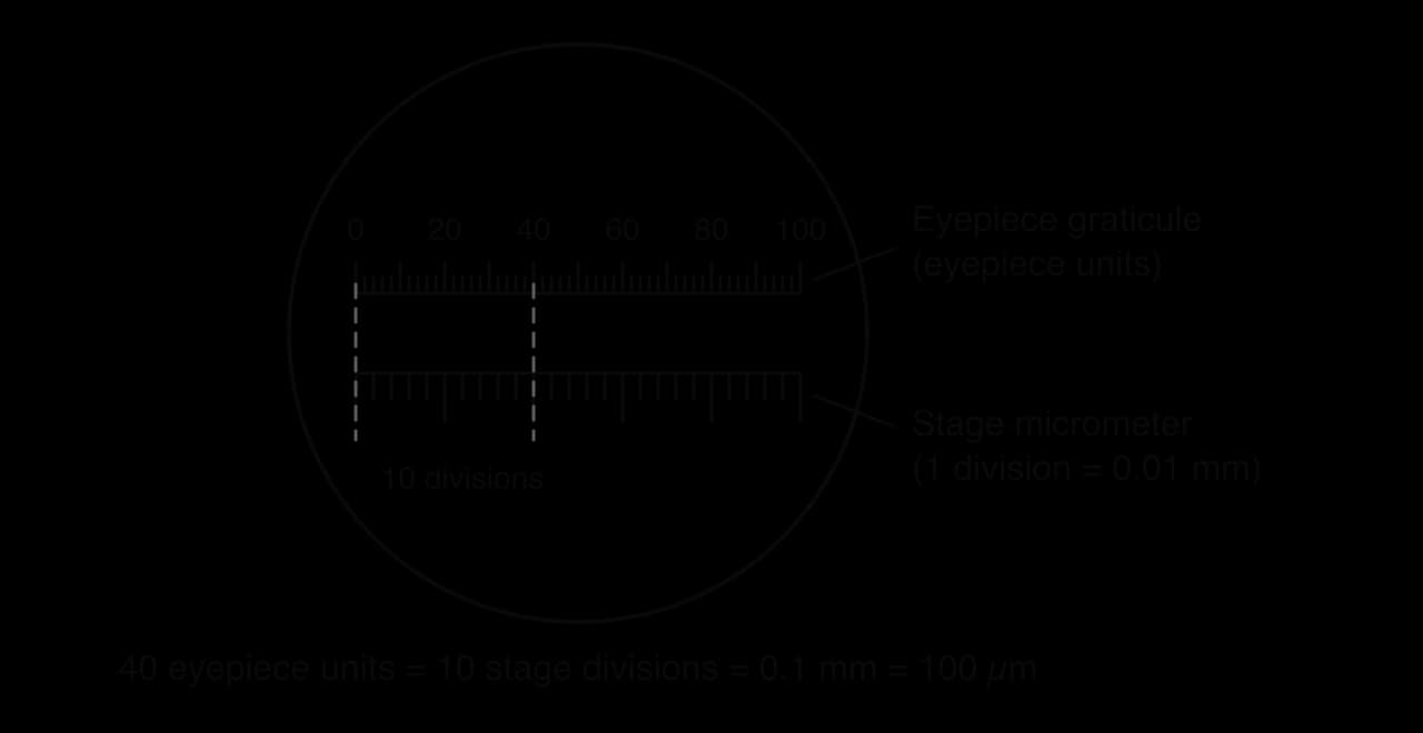
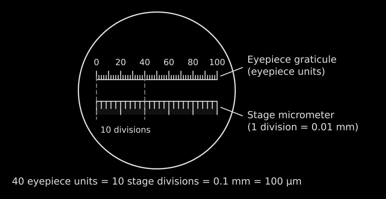
Microscopy and measurement of cells are taught in A2.2 Cell structure; magnification calculations are worked in Data, graphs and statistics.

Biological drawing

A biological drawing records what is seen in a specimen, accurately and clearly enough for another biologist to identify the structures. It shows the specimen actually observed, with its own shapes and proportions, and contains no structures that cannot be seen. Drawings are assessed on accuracy, clarity and the labelling of named features.

Conventions for a specimen drawing

• Use a sharp HB pencil and plain paper.

• Draw single, continuous lines; never sketch with many short strokes.

• Do not shade or colour. Show different regions with a line, or a few stipple dots where density matters.

• Draw what is seen, in correct proportion: if the nucleus is a fifth of the cell's width in the specimen, it is a fifth in the drawing.

• Make the drawing large, using at least half the space available.

• Rule label lines with a ruler, keep them horizontal where possible, make them end exactly on the structure, and never let them cross.

• Put labels outside the drawing, in a neat column, and never use arrowheads on label lines.

• Add a title naming the specimen, the stain if used, and the magnification or a scale bar.

The drawing of two onion epidermis cells meets every convention; the same cells drawn badly on the right show the most common faults side by side.

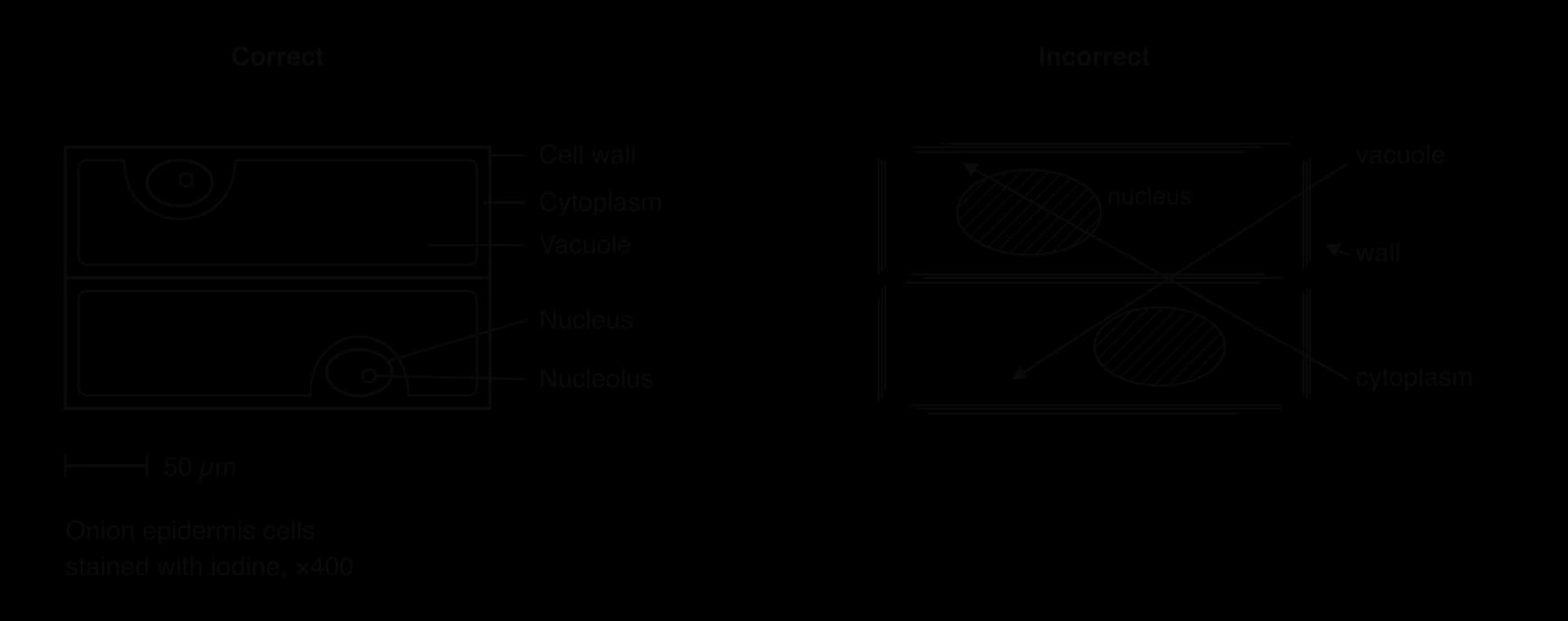
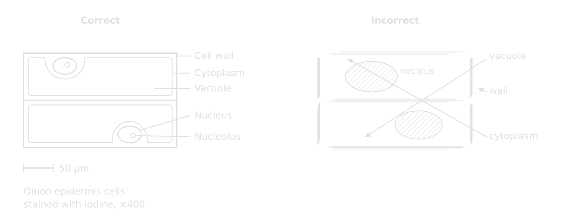
Drawing structures is part of A2.2 Cell structure (cells from micrographs) and of plant and animal tissue work in B3.1 Gas exchange and B3.2 Transport (leaf and stem sections).

Chromatography

Chromatography separates the substances in a mixture by how fast each moves through a stationary phase (paper, or a thin layer of silica gel on a plate) when carried by a solvent. A substance that is more soluble in the solvent and less attracted to the stationary phase moves further. In biology it is used to separate photosynthetic pigments, and also amino acids and sugars.

1. Draw a pencil line (the origin) about 2 cm from the bottom of the paper or plate. Pencil does not dissolve in the solvent; ink would.

2. Grind leaves with a little sand and propanone to extract the pigments.

3. Apply a small, concentrated spot of extract to the origin, letting each application dry before the next.

4. Stand the paper in a covered container with solvent below the origin, so the spot does not dissolve into the solvent.

5. Remove the paper before the solvent reaches the top, mark the solvent front at once and let it dry.

6. Measure the distance from the origin to the centre of each spot and to the solvent front.

Each substance has a characteristic Rf value for a given solvent and stationary phase. It is the ratio of the distance moved by the substance to the distance moved by the solvent, so it always lies between 0 and 1.

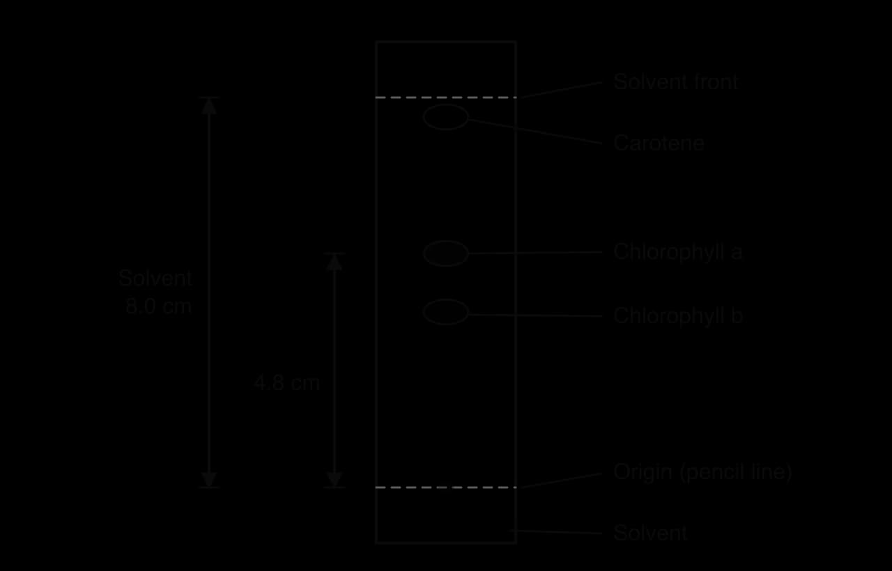
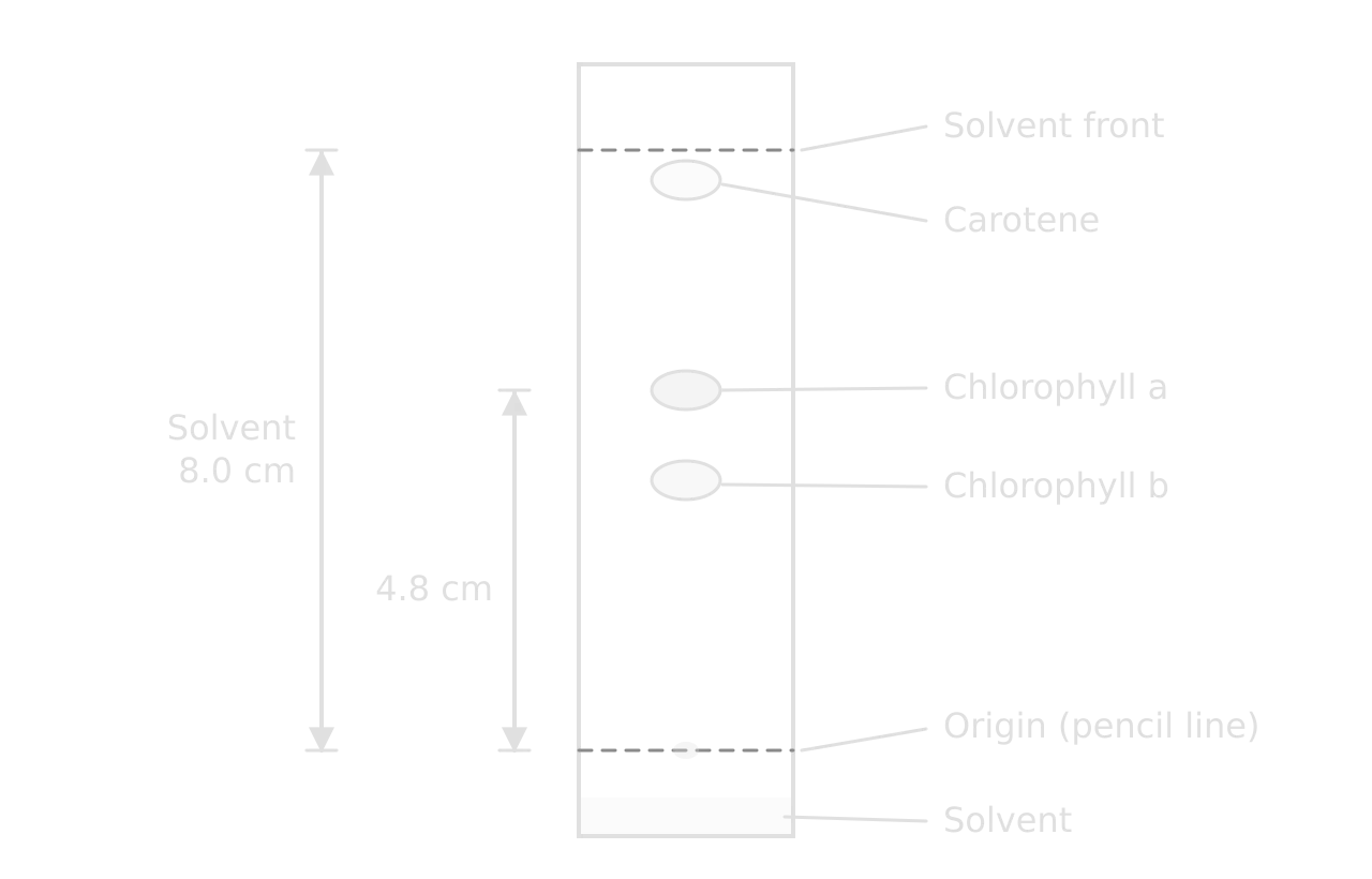
Chromatography of photosynthetic pigments is taught in C1.3 Photosynthesis, where the separated pigments are linked to the absorption spectrum.

Colorimetry and serial dilution

Colorimetry replaces judging colour by eye, which is subjective, with a measured value. A colorimeter shines light through a cuvette of solution and records the absorbance or the transmission. A filter or setting is chosen with the complementary colour of the solution, because that is the light the solution absorbs most: a red filter for a blue solution, for example.

Making a dilution series

To turn absorbance into concentration, a calibration curve is made from solutions of known concentration. These are prepared by serial dilution or by simple proportional dilution.

A serial dilution covers a wide range of concentrations quickly, but any error in one step is carried into every later step. For a narrower, evenly spaced range (0.2, 0.4, 0.6, 0.8 mol dm⁻³), each solution is made directly from the stock using $C_1{V}_1=C_2{V}_2$: for example, 8.0 cm³ of 1.0 mol dm⁻³ stock and 2.0 cm³ of water give 10 cm³ of 0.8 mol dm⁻³.

Using a calibration curve

The absorbance of each known solution is measured and plotted against concentration. The absorbance of the unknown sample is then read across to the line and down to the concentration axis.

Colorimetry is used to measure membrane damage from the leakage of beetroot pigment (B2.1 Membranes and membrane transport), the rate of starch digestion by amylase with iodine (C1.1 Enzymes and metabolism) and concentrations of reducing sugars.

Sampling methods in ecology

Populations are almost never counted in full. Instead, a sample is counted and the result scaled up. The method chosen depends on whether the organisms move and on the question being asked.

Random sampling avoids the bias of choosing quadrat positions by eye, which tends to favour the most interesting patches. Systematic sampling (at fixed intervals along a transect) is used instead when the aim is to follow a gradient, because random positions would miss parts of it.

Environmental variables along a transect (light, soil moisture, temperature) are measured with sensors and a data logger, so that the distribution of a species can be correlated with an abiotic factor.

Karyotyping

A karyotype is the number and appearance of the chromosomes in a cell; a karyogram is the image of those chromosomes arranged in pairs. Karyotyping is used to find the sex of an individual and to diagnose chromosome abnormalities.

1. Cells that can divide (white blood cells, or fetal cells from amniocentesis or chorionic villus sampling) are grown in culture.

2. Division is stopped at metaphase, when the chromosomes are most condensed.

3. The cells are burst on a slide, stained to show banding patterns and photographed.

4. The chromosomes are arranged in homologous pairs by size, centromere position and banding pattern, with the sex chromosomes last.

Karyotypes and karyograms are taught in A3.1 Diversity of organisms; the non-disjunction that causes trisomy is in D2.1 Cell and nuclear division.

Molecular modelling

Molecular models show the three-dimensional shapes of molecules, which are hard to see from a flat diagram. Physical models (ball-and-stick kits) are used to build molecules by hand and to act out reactions; digital models (molecular visualisation software such as Jmol or the viewers of the Protein Data Bank) display real structures determined by X-ray crystallography or cryo-electron microscopy.

• Building α- and β-glucose and joining two monomers by a condensation reaction, removing a water molecule (B1.1 Carbohydrates and lipids).

• Forming a dipeptide from two amino acids and identifying the peptide bond (B1.2 Proteins).

• Exploring the double helix of DNA and the structure of a nucleosome (A1.2 Nucleic acids).

• Rotating an enzyme to see the shape of its active site (C1.1 Enzymes and metabolism).

Every model is a simplification: ball-and-stick models exaggerate the spaces between atoms, and space-filling models hide the bonds. Questions on models often ask what a model shows well and what it leaves out.

Identification keys

A dichotomous key identifies an organism through a series of steps, each offering two contrasting descriptions. Choosing the description that fits leads either to a name or to the next step.

• Use features that are easy to see and do not vary within the species: number of legs, presence of a shell, leaf shape.

• Avoid relative or subjective terms such as "large", "dark" or "pretty".

• Make each pair of statements opposite versions of the same feature.

• A key for n organisms needs n − 1 steps.

At HL, designing a key for local species is part of A3.1 Diversity of organisms; cladogram analysis, a related skill, is in A3.2 Classification and cladistics.

Measuring variables

Every quantitative investigation depends on measuring the dependent variable accurately and controlling the others. The choice of instrument sets the uncertainty of each reading.

Qualitative data, such as colour changes or the presence of a structure, are recorded as descriptions; quantitative data are numbers with units. Where possible, a qualitative judgement (the colour of a solution) is replaced by a quantitative one (its absorbance in a colorimeter).

Safety and ethics

Safety of yourself, others and the environment

Every practical starts with a risk assessment: identify each hazard, judge the risk and state how it is reduced.

Ethics of working with organisms

Investigations must not cause pain, stress or lasting harm to any animal, vertebrate or invertebrate, and must follow the 3Rs: replace animals with alternatives (plants, microorganisms, simulations or databases) where possible, reduce the number used, and refine methods to minimise disturbance. In fieldwork, organisms are observed in place or returned where they were found, and habitats are left as they were.

Investigations on people need informed, written consent, the right to withdraw at any time, written consent from a parent or guardian for anyone under 16, no physical or psychological harm and anonymised data. Investigations involving body fluids, such as blood, are not allowed because of the risk of transmitting blood-borne pathogens; the only exception is investigators using their own saliva or sweat.