Data, graphs and statistics

Every mathematical tool used in biology data questions, from averages and standard deviation to t-tests, chi-squared and ecological indices, with worked examples.

IB Biology
Exam skills
SL and HL

19 min readLast reviewed 14 Oct 2026

Biology uses a small set of mathematical tools again and again: averages and spread, percentages and rates, magnification, correlation, a few statistical tests and two ecological indices. Each one appears in a particular subtopic, but any of them can be used in a Paper 1B or Paper 2 data question in a new context, and all of them are used in the internal assessment.

Each tool is set out with its formula, a worked example and the subtopic where it is first used. A calculator is allowed in both papers, so the skill being tested is choosing the right tool, setting out the working and interpreting the answer.

Averages: mean, median and mode

An average is a single value that represents a set of data. The three averages suit different kinds of data.

Average	How to find it	Best used when
Mean	Add all the values and divide by the number of values.	Data are continuous and roughly symmetrical, with no extreme values.
Median	Put the values in order and take the middle one (or the mean of the middle two).	Data are skewed or contain outliers.
Mode	The value that occurs most often.	Data are discrete or in categories, such as ABO blood groups.

Mean, median and mode are used together in D3.2 Inheritance to describe continuous variation, such as height, and the mean of quadrat counts is used in C4.1 Populations and communities.

Spread: range, interquartile range and box plots

Two data sets can have the same mean but very different spreads. The range (highest minus lowest value) is quick to find but depends on just two values, so a single outlier changes it. The interquartile range (IQR) is the spread of the middle half of the data: the upper quartile (Q3) minus the lower quartile (Q1). It is not affected by outliers.

A box-and-whisker plot shows the median, the quartiles and the range on one scale. The box runs from Q1 to Q3 with a line at the median; the whiskers run to the lowest and highest values that are not outliers. A common rule treats a value as an outlier if it is more than 1.5 × IQR below Q1 or above Q3.

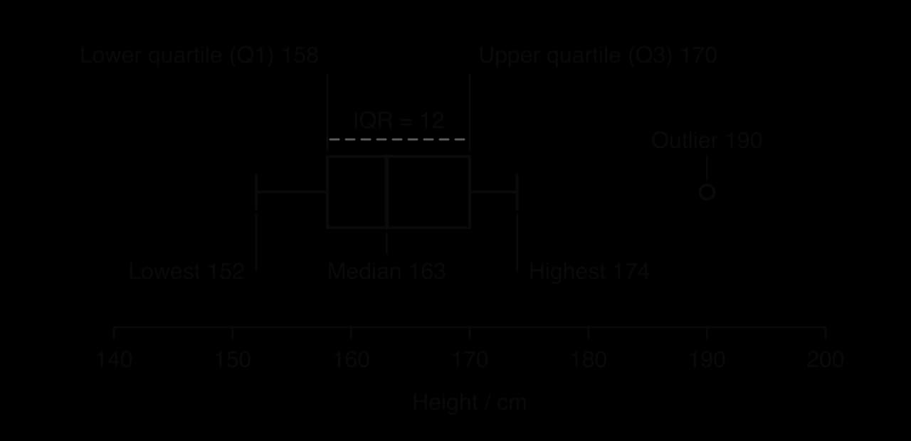
Box-and-whisker plot on a height axis from 140 to 200 cm. Box from lower quartile 158 to upper quartile 170 (IQR = 12) with the median at 163; whiskers to the lowest value 152 and highest value 174; an outlier plotted separately at 190. — Practice data: box plot of the heights of eleven students. The value of 190 cm is more than 1.5 × IQR above Q3, so it is plotted as an outlier and the whisker stops at 174 cm.

Box plots are used in D3.2 Inheritance to compare continuous variables between groups. When two box plots are compared, look at the medians, the overlap of the boxes and the spread.

Standard deviation

Standard deviation (SD) measures how spread out the values are around the mean. A small SD means the values are clustered close to the mean; a large SD means they vary widely. For data that follow a normal distribution, about 68% of values lie within one SD of the mean and about 95% within two SDs.

s = \sqrt{\frac{\sum (x - \overset{ˉ}{x})^{2}}{n - 1}}

In practice, SD is calculated with a calculator or spreadsheet. The formula is worth understanding once: each value's distance from the mean is squared, the squares are averaged (dividing by n − 1 for a sample) and the square root is taken.

Standard deviation is used in C4.1 Populations and communities to show the variation in quadrat counts, and in D2.3 Water potential to show the variation between repeats of mass-change measurements.

Standard error of the mean

The standard error (SE) of the mean shows how precisely a sample mean estimates the true mean of the population. It is the standard deviation divided by the square root of the sample size, so it falls as more measurements are taken.

SE = \frac{s}{\sqrt{n}}

Uncertainties and error bars

Measurement uncertainty

Every measurement has an uncertainty set by the instrument. For an analogue scale (a ruler, a measuring cylinder, a thermometer), it is usually half the smallest division. For a digital instrument, it is usually one unit of the last digit shown.

Instrument	Smallest division or digit	Uncertainty
Thermometer marked in 1 °C	1 °C	±0.5 °C
10 cm³ measuring cylinder marked in 0.2 cm³	0.2 cm³	±0.1 cm³
Ruler marked in mm	1 mm	±0.5 mm
Digital balance reading to 0.01 g	0.01 g	±0.01 g

The percentage uncertainty compares the uncertainty with the size of the reading. A ±0.5 mm uncertainty is 10% of a 5 mm measurement but only 1% of a 50 mm one, which is why longer measurements are more precise.

Error bars

An error bar is a line drawn above and below a plotted mean to show the spread or uncertainty of the data. It may show the range, ±1 SD or ±1 or 2 SE, and the graph or its caption must say which. Error bars are read in two ways: their length shows how variable the repeats were, and their overlap suggests whether two means are likely to be different.

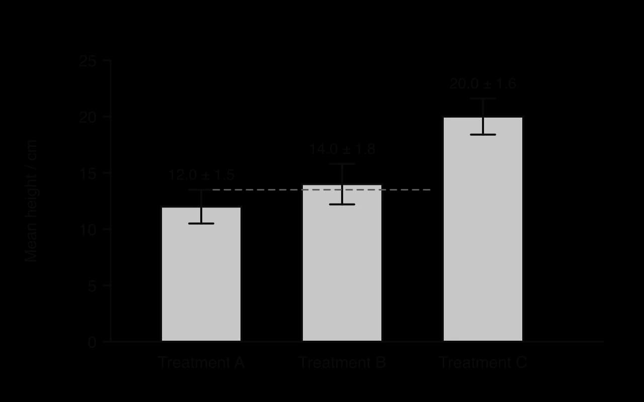
Error bars are used in D2.3 Water potential, where the means of repeated mass-change measurements are plotted against solution concentration.

Percentage change and percentage difference

Percentage change compares the same quantity at two times, relative to its starting value. Percentage difference compares two values measured at the same time, such as cases of a disease in two countries, relative to their mean.

% change = \frac{final value - initial value}{initial value} \times 100

% difference = \frac{∣ a - b ∣}{(a + b) \div 2} \times 100

Both are used in C3.2 Defence against disease to compare data on the COVID-19 pandemic between countries and over time, and percentage change is used in D4.2 Stability and change to measure deforestation.

Rates and gradients

A rate is a change divided by the time it took, so its unit always contains "per unit time" (cm³ s⁻¹, mm day⁻¹, beats min⁻¹). A mean rate over a period is the total change divided by the total time. On a graph of a quantity against time, the rate at any moment is the gradient of the curve at that point, found by drawing a tangent.

For an enzyme reaction, the rate of reaction is fastest at the start, when substrate concentration is highest, so the initial rate is found from a tangent drawn at time zero.

Product formed
Tangent at t = 0

General shape of product formed against time in an enzyme reaction. The tangent at t = 0 rises 20 cm³ in 4 min, so the initial rate is 5 cm³ min⁻¹; the curve flattens as substrate is used up.

Rates and tangents are used in C1.1 Enzymes and metabolism, and rates of gas production or uptake in C1.2 Cell respiration and C1.3 Photosynthesis.

Magnification and scale bars

Magnification is how many times larger an image is than the real object. Image size and actual size must be in the same unit before dividing.

magnification = \frac{image size}{actual size}

Unit	In metres	Conversion
millimetre (mm)	10⁻³ m	1 mm = 1000 µm
micrometre (µm)	10⁻⁶ m	1 µm = 1000 nm
nanometre (nm)	10⁻⁹ m	1 nm = 0.001 µm

A scale bar is a line on a micrograph labelled with the actual length it represents. Because it is enlarged with the image, it gives the magnification even when the image is printed at a different size.

Magnification, scale bars and measurement with an eyepiece graticule are taught in A2.2 Cell structure; graticule calibration is set out in Practical techniques and biological drawing.

Correlation, r and R²

A correlation is a relationship between two variables in which one tends to change as the other changes. In a positive correlation both increase together; in a negative correlation one decreases as the other increases. A scatter graph with a line of best fit shows the pattern.

Line of best fit

Practice data set: number of plants of one species per quadrat against light intensity in ten quadrats along a transect. The points lie close to the line: r = 0.986, R² = 0.97.

The strength of a straight-line correlation is measured by the correlation coefficient, r, which runs from −1 (perfect negative) through 0 (no correlation) to +1 (perfect positive). The coefficient of determination, R², is the square of r. It gives the proportion of the variation in one variable that is explained by the other: R² = 0.97 means that 97% of the variation in plant number is accounted for by the variation in light intensity.

Correlation and causation

A correlation does not show that one variable causes the change in the other. A third, confounding variable may cause both, or the link may be coincidence. In the quadrat data, more light could cause more plants, but light-rich quadrats might also have drier soil or less trampling. Causation is shown by a controlled experiment in which only the independent variable is changed, or by a known mechanism supported by several independent studies.

The correlation coefficient is used in B3.2 Transport to analyse data on risk factors for coronary heart disease, and R² in C2.2 Neural signalling for the relationship between axon diameter and the speed of nerve impulses.

Hypotheses and statistical significance

Statistical tests are used to decide whether a pattern in data is likely to be real or could be due to chance. Each test starts with two hypotheses.

The null hypothesis (H₀) states that there is no difference between groups, or no association between variables.
The alternative hypothesis (H₁) states that there is a difference or an association.

The test produces a value (t or χ²) that is compared with a critical value from a table, at a chosen significance level, usually p = 0.05. If the calculated value is greater than the critical value, p is less than 0.05: there is less than a 5% probability that a difference this large would arise by chance if H₀ were true. The null hypothesis is then rejected and the result is statistically significant.

The t-test

A t-test compares the means of two groups of continuous data to see whether they are significantly different. It assumes the data are roughly normally distributed. Degrees of freedom for two independent groups are $n_{1} + n_{2} - 2$ .

t = \frac{{\overset{ˉ}{x}}_{1} - {\overset{ˉ}{x}}_{2}}{\sqrt{\frac{s_{1}^{2}}{n_{1}} + \frac{s_{2}^{2}}{n_{2}}}}

The chi-squared test

The chi-squared test (χ²) compares observed frequencies (counts in categories) with the frequencies expected if the null hypothesis were true. It is used on counts, never on means, percentages or measurements.

χ^{2} = \sum \frac{(O - E)^{2}}{E}

In a test for association between two species, quadrats are scored for the presence or absence of each species, and the counts are set out in a 2 × 2 contingency table. The expected frequency for each cell is (row total × column total) ÷ grand total. Degrees of freedom are (rows − 1) × (columns − 1), which is 1 for a 2 × 2 table, with a critical value of 3.84 at p = 0.05.

In 100 quadrats, species A and B were both present in 30, A only in 10, B only in 15 and neither in 45. Calculate χ² and deduce whether the two species are associated. [4]

Show the solution

Totals: A present 40, A absent 60; B present 45, B absent 55. Expected values:

	B present	B absent	Row total
A present	O = 30, E = 40 × 45 ÷ 100 = 18	O = 10, E = 40 × 55 ÷ 100 = 22	40
A absent	O = 15, E = 60 × 45 ÷ 100 = 27	O = 45, E = 60 × 55 ÷ 100 = 33	60
Column total	45	55	100

χ^{2} = \frac{12^{2}}{18} + \frac{12^{2}}{22} + \frac{12^{2}}{27} + \frac{12^{2}}{33} = 8.00 + 6.55 + 5.33 + 4.36 = 24.2

Expected values correct [1]; χ² = 24.2 [1].
df = 1; 24.2 > 3.84, so p < 0.05 and H₀ (no association) is rejected [1].
The species occur together more often than expected (30 observed, 18 expected), so the association is positive [1].

The test for association between species is used in C4.1 Populations and communities. At HL, D3.2 Inheritance uses the same test to compare the observed offspring of a dihybrid cross with the expected 9:3:3:1 ratio, with 3 degrees of freedom (critical value 7.81).

Ecological indices

Simpson's reciprocal index

Simpson's reciprocal index (D) measures the diversity of a community from the number of individuals of each species. It takes into account both species richness and species evenness. Its lowest value is 1 (one species only), and a higher value means a more diverse community.

D = \frac{N (N - 1)}{\sum n (n - 1)}

N is the total number of individuals of all species and n is the number of individuals of each species.

Simpson's reciprocal index is used in A4.2 Conservation of biodiversity to compare the diversity of habitats.

The Lincoln index

The Lincoln index estimates the size of a population of motile animals by capture–mark–release–recapture. A sample is caught, marked and released; later a second sample is caught and the marked individuals in it are counted.

N = \frac{M \times n}{m}

M is the number caught and marked in the first sample, n the total caught in the second sample and m the number of marked individuals recaptured.

The Lincoln index is used in C4.1 Populations and communities, alongside random quadrat sampling for plants and other sessile organisms.

Logarithmic scales

A logarithmic scale increases by equal multiples rather than equal steps: each major division is ten times the one before (1, 10, 100, 1000). It is used when data cover several orders of magnitude, such as bacterial numbers or body masses. On a log scale, exponential growth plots as a straight line, which makes it easy to recognise.

Bacterial population

A population of 100 bacteria doubling every 20 minutes, plotted as log₁₀ of cell number. Exponential growth gives a straight line; each unit up the y-axis is a tenfold increase.

Logarithmic scales are used in C4.1 Populations and communities to test whether population growth fits an exponential model.

Choosing the right tool

Question about the data	Tool	First used in
What is a typical value?	Mean, median or mode	C4.1, D3.2
How variable are the values?	Range, IQR, standard deviation	C4.1, D3.2
How precise is the mean?	Standard error	D2.3
How much did a value change?	Percentage change	C3.2, D4.2
How different are two values at the same time?	Percentage difference	C3.2
How fast did it change?	Rate, gradient, tangent	C1.1
How large is it really?	Magnification, scale bar	A2.2
Are two variables related?	Scatter graph, r, R²	B3.2, C2.2
Are two means significantly different?	t-test	Internal assessment
Do observed counts differ from expected?	Chi-squared	C4.1; D3.2 (HL)
How diverse is a community?	Simpson's reciprocal index	A4.2
How many animals are there?	Lincoln index	C4.1

Write the formula in words or symbols.
Substitute the values with units.
Give the answer with a unit and sensible precision (usually as many significant figures as the data).
Interpret the answer in the context of the question.

Carry on with Biology in Augment

With a free account, Augment remembers where you stopped in the notes and which questions you have marked.

Start free