2 Functions

Introduction

A function is a rule that gives exactly one output for each input: the cost of a taxi ride for each distance, the height of a tide at each hour, the population of a country in each year. Topic 2 studies functions in three linked representations, the equation, the table of values and the graph, and uses technology to move between them. Its aim is practical. A function is chosen to describe a real situation, fitted to data, and then used to answer a question.

This makes functions the language of modelling for the whole course. A mathematical model is useful only where it fits reality well, so the topic also teaches how to test a model, where it can be trusted, and why predictions far outside the data are risky. At HL the range of models widens, and functions can be combined, reversed and transformed.

YouTube

How the subtopics fit together

The subtopics form two strands. The map of the topic shows each strand as a row, with the SL subtopics shaded and the HL-only subtopics dashed; an arrow means the first subtopic is used in the second.

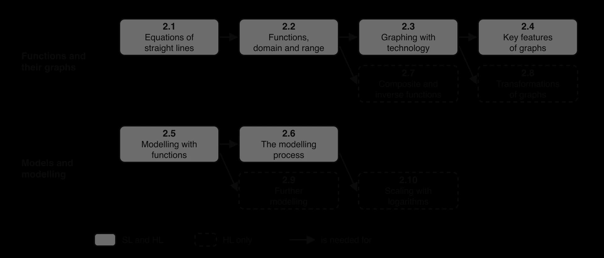
The functions and their graphs strand starts from the straight line, the simplest function, with its gradient as a rate of change. Function notation, domain and range follow, then graphing with a GDC and reading off the key features: intercepts, zeros, maximum and minimum points, asymptotes and points of intersection. Solving an equation by finding where two graphs meet is the method used throughout the course when algebra alone would be slow.

The models and modelling strand applies these skills. Subtopic 2.5 builds the families of models, and subtopic 2.6 turns the work into a cycle: state assumptions, fit the parameters, test the model against data, reflect on its limitations and use it. At HL the strand adds logistic, natural logarithmic, phase-shifted sinusoidal and general piecewise models, and logarithms straighten curved data so that an exponential or a power model can be chosen and fitted.

The subtopics

Links to other topics

Functions connect to every other topic. Exponential models are the continuous form of the geometric sequences and compound interest of topic 1, and the GDC's equation solvers from subtopic 1.8 find a model's parameters from given points. Fitting a model to data by regression belongs to topic 4: linear regression in subtopic 4.4 and, at HL, curved models with $R^2$ in subtopic 4.13.

Calculus in topic 5 analyses the same functions: the derivative is used to find where a model reaches its maximum, and the integral gives the area under its graph. Sinusoidal models use the trigonometry of topic 3, with angles in degrees at SL and radians at HL (subtopic 3.7).