2.5 Modelling with functions

Introduction

A function becomes a model when its input and output stand for real quantities: time and temperature, distance and height, price and profit. A small set of function families covers a wide range of situations, because each family describes one particular pattern of change. A constant rate of change gives a straight line, a constant percentage change gives an exponential curve, a repeating cycle gives a sine curve, and a quantity that rises to a peak and falls again is often quadratic. Knowing the shape, the formula and the meaning of the numbers in each family makes it possible to recognise which one fits a situation and to calculate with it.

The same few families appear across the sciences and social sciences: exponential decay for medicines leaving the bloodstream and hot drinks cooling, inverse variation for gases being compressed, the cube of wind speed for the power of a wind turbine, and sine curves for tides and Ferris wheels.

Functions as models

A mathematical model describes a real situation with a function, so that questions about the situation become questions about the function. The input is usually the independent variable (often time $t$ or a distance $x$) and the output is the dependent variable being predicted. Every model family has a general formula containing letters that are fixed for one particular situation but change from one situation to another.

Parameters usually have a physical meaning and units. In a model of a car's value, one parameter might be the price when new, in dollars, and another the fraction of value kept each year, with no units. Interpreting a parameter means saying exactly what it represents in the situation, with its units. Finding a parameter means using given information (a point the graph passes through, a maximum, a starting value) to calculate it.

The six families used for SL models, with the pattern each one describes, are summarised in the table.

Linear models

A quantity that changes by the same amount for every unit increase in the input has a constant rate of change, and its graph is a straight line. Subtopic 2.1, Equations of straight lines, gives the algebra of lines; a linear model adds the meaning of each number.

The two parameters have fixed roles in any context.

• The gradient $m$ is the rate of change: the change in the output for each one-unit increase in the input. Its units are "output units per input unit" (dollars per day, centimetres per hour). A positive $m$ means the quantity increases; a negative $m$ means it decreases.

• The y-intercept $c$ is the value of the output when the input is 0: a fixed charge, a starting amount or a starting height. Its units are the output's units.

A linear model is justified by its constant rate: the value at $x + 1$ minus the value at $x$ is $m(x + 1) + c - (mx + c) = m$, whatever $x$ is. A table of values with equally spaced inputs and constant differences in the outputs is therefore a strong sign that a linear model fits.

The interpretation of $c$ must be specific to the context. A phrase such as "the starting value" could describe any model, while "the fixed charge of $40 paid before any days of hire" says what the number actually is.

Building a linear model from two data points

When two points on the line are known, the gradient formula from subtopic 2.1 gives $m$, and substituting either point gives $c$. The model can then be used for prediction within a sensible domain.

Piecewise linear models

Many real charges and shapes follow one straight line for part of the domain and a different straight line for another part. A mobile phone plan may charge a flat fee up to a data allowance and a rate per gigabyte beyond it; the floor of a swimming pool may be level, then slope down, then level again.

A piecewise linear model is written with a brace, listing each linear piece with the interval on which it applies. The intervals must not overlap, so that every input has exactly one output, and together they cover the whole domain. In most real contexts the pieces join where one interval ends and the next begins, so the graph is one unbroken line with corners.

A swimming pool is 25 m long. The floor is level at a depth of 1.0 m for the first 6 m from the shallow end, then slopes down steadily to a depth of 3.0 m at 16 m from the shallow end, and is level from there to the deep end. With $x$ the distance in metres from the shallow end, the depth $D$ in metres is:

The middle piece falls 2.0 m in depth over 10 m of length, so its gradient is $\frac{2.0}{10} = 0.2$ metres of depth per metre along the pool. Writing it as $1.0 + 0.2(x - 6)$ makes it start at the right value: at $x = 6$ it gives 1.0, the depth where the slope begins, and at $x = 16$ it gives $1.0 + 0.2 \times 10 = 3.0$.

The graph of the depth model shows three straight pieces joined at corners. A depth of 2.5 m occurs only on the sloping piece, which is why the point $(13.5, 2.5)$ is found from the middle formula: $1.0 + 0.2(x - 6) = 2.5$ gives $x = 13.5$.

Another common context is an object moving towards and then away from a wall at constant speeds: its distance from the wall decreases linearly, may stay constant while it pauses, then increases linearly. The gradient of each piece is the velocity on that stage, negative when approaching and positive when moving away.

Quadratic models

A quantity that rises to a single maximum and then falls symmetrically (or falls to a single minimum and rises again) is often modelled by a quadratic. A ball thrown into the air, the arch of a bridge, the area of a field enclosed by a fixed length of fence and the profit from selling at different prices all behave this way.

The graph of every quadratic has the same basic shape, which is named separately because it appears in so many applications.

The sign of $a$ controls the direction: when $a > 0$ the parabola opens upwards and has a lowest point, and when $a < 0$ it opens downwards and has a highest point. The size of $a$ controls how narrow the curve is: a larger $|a|$ gives a steeper, narrower parabola. The constant $c$ is the y-intercept, because $f(0) = a \times 0 + b \times 0 + c = c$.

Axis of symmetry and vertex

Every parabola is symmetrical about a vertical line, and the turning point lies on that line.

The formula can be justified without calculus. The points on the parabola at the height of the y-intercept, $y = c$, satisfy $ax^2 + bx + c = c$, which simplifies to $x(ax + b) = 0$. So the parabola is at height $c$ when $x = 0$ and when $x = -\frac{b}{a}$. Two points at the same height on a symmetrical curve lie equal distances either side of the axis, so the axis is exactly halfway between them.

The turning point on the axis has its own name.

To find the vertex, find its x-coordinate from $x = -\frac{b}{2a}$, then substitute that value into the function for the y-coordinate. On a GDC the vertex can also be read with the maximum or minimum tool (subtopic 2.4, Key features of graphs, describes these tools); when the function is given with numerical coefficients, the formula gives an exact x-coordinate and a working that can be checked.

Zeros and intercepts

The zeros of a quadratic, where $f(x) = 0$, are the x-intercepts of the parabola and the roots of the equation $ax^2 + bx + c = 0$. A parabola can cross the x-axis twice, touch it once at the vertex, or miss it altogether, so a quadratic has two, one or no real zeros. Because of the symmetry, two zeros always lie equal distances either side of the axis: their mean is $-\frac{b}{2a}$. The zeros are found with the GDC, either with the zero (root) tool on the graph or with the polynomial equation solver (subtopic 1.8, Equations and systems using technology).

The four features fit together on one graph. A ball is thrown upwards from a balcony; its height $h$ metres after $t$ seconds is modelled by $h(t) = -4.9t^2 + 14.7t + 2$.

The graph of the ball's height shows the y-intercept 2 (the height of the balcony), the vertex on the axis of symmetry, and two zeros. Only the positive zero has meaning: the negative one is a time before the ball was thrown, outside the reasonable domain of the model.

Finding the parameters of a quadratic

A quadratic has three parameters, so three independent pieces of information fix it. These can be three points, or a vertex (which gives a point and the axis of symmetry) and one more point, or two zeros and the vertex. Each piece of information becomes a linear equation in $a$, $b$ and $c$; the resulting system of linear equations is solved with the GDC's simultaneous equation solver.

• A point $(p, q)$ on the graph gives $ap^2 + bp + c = q$.

• A y-intercept $q$ gives $c = q$ directly.

• An axis of symmetry $x = s$ gives $-\frac{b}{2a} = s$, which rearranges to the linear equation $b = -2as$

Optimising with a quadratic

Because the vertex of a parabola is its highest or lowest point, a quadratic model gives the best possible value of a quantity directly. A farmer has 200 m of fencing to make a rectangular pen against a long wall, so only three sides need fencing. If the two sides at right angles to the wall are $x$ m long, the side parallel to the wall is $200 - 2x$ m, and the area is

The axis of symmetry is $x = -\frac{200}{2 \times (-2)} = 50$, so the largest area is $A(50) = 50 \times 100 = 5000\text{ m}^2$, with the side along the wall 100 m long. The reasonable domain is $0 < x < 100$, because both lengths must be positive. Problems like this are extended to other functions with calculus in subtopic 5.7, Optimisation.

Exponential models

When a quantity is multiplied by the same factor in every equal time interval, it changes by a constant percentage rather than a constant amount. A population growing by 4% a year, a medicine of which 18% leaves the body each hour, and the value of a car falling by 15% a year all behave this way. Subtopic 1.3, Geometric sequences and series, treats this as a sequence of values at whole-number steps; an exponential model describes the same pattern as a continuous function of time.

The model $f(x) = ka^x + c$

The general exponential model has three parameters. The base $a > 0$ is the growth factor per unit of $x$: growth when $a > 1$ and decay when $0 < a < 1$ (a decay factor). The constant $c$ shifts the whole graph up or down, and $k$ scales it.

The ratio idea explains the name. When $c = 0$, $\frac{f(x + 1)}{f(x)} = \frac{ka^{x+1}}{ka^x} = a$: every increase of 1 in $x$ multiplies the output by $a$. A percentage change of $r\%$ per unit therefore gives $a = 1 + \frac{r}{100}$ for growth and $a = 1 - \frac{r}{100}$ for decay. A decay factor of 0.82 means 82% remains after each unit of time, so 18% is lost.

The table of a medicine model shows the defining property: the differences between consecutive values shrink (7.2, then 5.9, then 4.8, …), but the ratios stay at 0.82.

Initial value. When $x = 0$, $a^0 = 1$, so $f(0) = k + c$.

Horizontal asymptote. For a decay model ($0 < a < 1$), $a^x$ gets closer and closer to 0 as $x$ increases, but never reaches it. So $ka^x + c$ gets closer and closer to $c$ without reaching it, and the graph has the horizontal asymptote $y = c$. For a growth model the same line is approached as $x$ becomes large and negative. In context, $y = c$ is the long-run value of a decaying quantity: the room temperature a drink cools towards, or the smallest population a model allows.

The direction of approach depends on the sign of $k$. When $k > 0$ the curve lies above the asymptote; when $k < 0$ it lies below it, and a decay model then rises towards $c$, as the speed of a falling object rises towards a terminal speed.

The graph of a growth curve and a decay curve with the same $c = 2$ shows both features together. Each y-intercept is $k + c$, and both curves flatten towards $y = 2$, on opposite sides of the y-axis.

Logarithms do give an exact method: $0.82^t = 0.125$ means $t = \frac{\log 0.125}{\log 0.82}$ (subtopic 1.5, Exponents and introduction to logarithms). Because a GDC is always to hand, the graphical or solver method is quicker and less error-prone, and it works equally well for models such as $21 + 67(0.94)^t = 60$ where logarithms need extra rearranging.

The form $f(x) = ka^{-x} + c$

A negative exponent turns growth into decay. Because $a^{-x} = \left(\frac{1}{a}\right)^x$, the model $ka^{-x} + c$ with $a > 1$ is a decay model with decay factor $\frac{1}{a}$. The model $P = 1200 + 500(1.25)^{-t}$, for example, decays by a factor $\frac{1}{1.25} = 0.8$ each unit of time, starts at $1200 + 500 = 1700$ and approaches 1200. Both forms appear in practice, so the decay factor and the percentage lost should be found from $\frac{1}{a}$ when the exponent is negative.

When $c \ne 0$, the constant percentage change applies to the distance from the asymptote, $ka^{-x}$, and not to the whole value. In the model $P = 1200 + 500(1.25)^{-t}$, the part above 1200 falls by 20% each unit of time, while $P$ itself falls by a smaller and smaller percentage.

Newton's law of cooling

A hot drink left in a room cools quickly at first and then more and more slowly. Newton's law of cooling states that the rate of heat loss is proportional to the difference between the object's temperature and its surroundings. The result is that the temperature difference decays exponentially, so the temperature itself follows $T = c + ka^t$, where $c$ is the room temperature (the asymptote) and $k$ is the starting difference.

The form $f(x) = k\mathrm{e}^{rx} + c$

Many scientific models use the base e ≈ 2.718 (subtopic 1.5). Here the sign of $r$ decides the behaviour: $r > 0$ gives growth and $r < 0$ gives decay. The model is still exponential in the same sense, because $\mathrm{e}^{rx} = \left(\mathrm{e}^r\right)^x$, so the growth factor per unit is $a = \mathrm{e}^r$. A model $P = 500\mathrm{e}^{0.05t}$ grows by a factor $\mathrm{e}^{0.05} = 1.0513\ldots$ per unit of time, about 5.13% each time. The initial value is $k + c$, as before, and the asymptote is $y = c$.

The exponential model is the continuous version of the discrete models in topic 1: geometric sequences (1.3), compound interest and depreciation (1.4), and loans and annuities (1.7). The time for an exponentially decaying quantity to halve is its half-life; with a GDC it is found by solving $ka^t = \frac{1}{2}k$.

No exponential growth continues for ever. A population growing by a constant percentage eventually exceeds the space or food available, so an exponential growth model is usually valid only over a limited domain; predicting far beyond the data is extrapolation, whose dangers are discussed in subtopic 2.6.

Direct and inverse variation

Some quantities are linked by a power: the area of a square varies with the square of its side, the power of a wind turbine with the cube of the wind speed, and the pressure of a gas with the reciprocal of its volume. These are modelled by $f(x) = ax^n$, where $n$ is an integer and $a$ is a constant.

The constant $a$ has its own name, because finding it is the first step of every variation problem.

Properties of direct variation

For $n > 0$, the graph of $y = ax^n$ passes through the origin, because $y = 0$ when $x = 0$. The most useful property is the scaling rule: multiplying $x$ by a factor $s$ multiplies $y$ by $s^n$, since

So if $y \propto x^2$, doubling $x$ multiplies $y$ by 4; if $y \propto x^3$, doubling $x$ multiplies $y$ by 8. The case $n = 1$, $y = ax$, is a linear model through the origin.

The theoretical power of a wind turbine increases as the cube of the wind speed, $P \propto v^3$. A wind that is twice as fast carries $2^3 = 8$ times as much power. Real turbines are controlled so that their output stays at a fixed rated power once the wind is strong enough, to protect the machinery, so $P = kv^3$ describes only the range of speeds below that rated speed.

Inverse variation

When $n$ is a negative integer, $y = ax^n = \frac{a}{x^{|n|}}$: as $x$ increases, $y$ decreases. This is inverse variation.

For inverse variation with $n = 1$, the product $xy$ is constant: doubling one quantity halves the other. Boyle's law for a fixed amount of gas at constant temperature is an example: the pressure $p$ and volume $V$ satisfy $pV = \text{constant}$, so $p = \frac{k}{V}$. Squeezing a gas into half the volume doubles its pressure.

The graphs of inverse variation have two asymptotes, both on the axes.

• The function is undefined at $x = 0$ (division by zero), and as $x$ approaches 0 the values of $y$ grow without limit. The y-axis, $x = 0$, is a vertical asymptote.

• As $x$ becomes very large, $\frac{a}{x^n}$ becomes very small but never 0. The x-axis, $y = 0$, is a horizontal asymptote.

The graph of $y = \frac{2}{x}$ and $y = \frac{2}{x^2}$ shows both asymptotes. With an odd power the two branches lie in opposite quadrants; with an even power both lie above the x-axis, because $x^2$ is never negative. In most real contexts only $x > 0$ has meaning (volumes, distances), so only the right-hand branch is drawn.

The inverse square law

Light, sound and gravity all spread out from a source. Energy leaving a small source in every direction is spread over the surface of a sphere, of area $4\pi d^2$ at distance $d$, so the intensity (energy per square metre) varies as $\frac{1}{d^2}$.

Doubling the distance from a lamp quarters the light falling on each square metre; tripling it divides the intensity by 9.

Cubic models

A cubic function can rise, fall and rise again (or the reverse), so it suits quantities with a peak and a trough, such as the volume of a box made by cutting corners from a sheet, or the height profile of a road over a hill and into a valley.

Features of cubic graphs

The graph of a cubic has at most two turning points (one local maximum and one local minimum) and at most three zeros. It always has at least one zero, because the $ax^3$ term dominates for large $|x|$: when $a > 0$, $f(x)$ is large and negative for large negative $x$ and large and positive for large positive $x$, so the graph must cross the x-axis somewhere. When $a < 0$ the ends are the other way round. The y-intercept is $d$, because $f(0) = d$. Between the two turning points the curve changes the direction in which it bends.

These features are the evidence for choosing a cubic: a graph or data set with one local maximum and one local minimum, or with three zeros, suggests a cubic model. "It looks like an S" is too vague to justify the choice.

The zeros of a cubic are found with the GDC's polynomial solver or the zero tool; its turning points with the maximum and minimum tools.

Finding the parameters of a cubic

A cubic has four parameters, so four pieces of information are needed. If one of the points is the y-intercept, it gives $d$ at once, leaving three equations in $a$, $b$ and $c$ for the GDC's solver.

The graph of the path model shows why part (c) checks the end points: on a restricted domain the highest or lowest value of a function can occur at an end rather than at a turning point. Here both turning points are more extreme than the ends.

Sinusoidal models

Tides, the height of a seat on a Ferris wheel, hours of daylight and seasonal temperatures repeat in regular cycles. Their graphs look like the graphs of sine and cosine, stretched and moved, and the functions that model them are called sinusoidal.

Sine and cosine take values between −1 and 1 and repeat every 360°. The graph of $y = \sin x$ starts at 0, rises to 1 at 90°, returns to 0 at 180°, falls to −1 at 270° and is back at 0 at 360°. The graph of $y = \cos x$ has the same shape but starts at its maximum, 1, at $x = 0$. The three parameters stretch and move these curves, and each has a name.

The amplitude is always a positive number, a distance. For a model with known maximum and minimum values:

The formula follows from the basic curve. $\sin(bx)$ completes one cycle when $bx$ runs from 0° to 360°, which is when $x$ runs from 0 to $\frac{360}{b}$. So multiplying $x$ by $b$ squeezes the cycle by a factor $b$: $b = 2$ gives a period of 180°, and $b = 30$ a period of 12. To find $b$ from a known period, rearrange.

The maximum value of the model is $d + |a|$ and the minimum is $d - |a|$.

The graph of a buoy's height above the sea bed, $y = 0.6\sin(45t) + 4$, shows all three features: the curve oscillates between 3.4 m and 4.6 m (amplitude 0.6), about the principal axis $y = 4$, and one full cycle takes $\frac{360}{45} = 8$ seconds.

Choosing sine, cosine or negative cosine

With the input in degrees and no horizontal shift, the choice of function is fixed by what happens at $x = 0$.

The negative cosine model $-a\cos(bx) + d$ is the same family with a negative first parameter; the amplitude is still the positive number $a$.

The depth in part (c) is above 7 m around each high tide, so the time is split between the start and the end of the cycle; by symmetry it is twice 2.311 hours. A sketch of the graph with the line $y = 7$ makes this clear, and is worth drawing before solving.

Case study: The London Eye

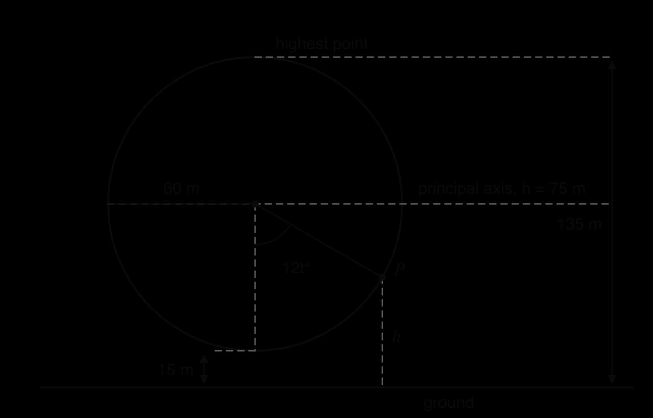
The London Eye on the South Bank of the Thames is a giant observation wheel. The structure is 135 m tall, the wheel has a diameter of 120 m, and it turns slowly enough that one revolution takes about 30 minutes. The height of a point on the rim is a sinusoidal function of time, and its parameters come straight from the geometry.

Source: Wikipedia, "London Eye", accessed 2026.

Model a point $P$ on the rim that is at its lowest position at $t = 0$, with the assumption that the top of the rim is at the full height of the structure, 135 m. The radius is 60 m, so the centre of the wheel is $135 - 60 = 75$ m above the ground and the lowest point of the rim is $75 - 60 = 15$ m above it. The diagram of the wheel shows these heights and the angle through which $P$ has turned.

The three parameters each match a feature of the wheel.

• Amplitude: the point moves 60 m above and below the centre, so the amplitude is the radius, 60 m.

• Principal axis: the centre height, $h = 75$.

• Period: 30 minutes, so $b = \frac{360}{30} = 12$. In one minute the wheel turns 12°, which is why the angle in the diagram is $12t$ degrees.

Starting at the lowest point means a negative cosine: $h(t) = -60\cos(12t) + 75$, with $t$ in minutes and $h$ in metres. The diagram also gives a direct justification. When $P$ has turned through $12t$ degrees from the bottom, it is $60\cos(12t)$ metres below the centre (right-angled trigonometry in the triangle under the centre), so its height is $75 - 60\cos(12t)$. Once $P$ passes the level of the centre, $\cos(12t)$ is negative and the same expression places $P$ above the centre, so one formula covers the whole revolution.

Typical questions about the wheel can be answered from the model and its graph over one revolution.

• Height after 5 minutes: $h(5) = -60\cos(60^\circ) + 75 = -30 + 75 = 45$ m.

• Time above 100 m in each revolution: solving $-60\cos(12t) + 75 = 100$ with the GDC (degree mode) gives $t = 9.552\ldots$ and $t = 20.447\ldots$, so the point is above 100 m for $20.447\ldots - 9.552\ldots = 10.9$ minutes, just over a third of each revolution.

The model has limitations. The capsules are mounted on the outside of the rim, so the height of a passenger's floor is not exactly the height of a rim point: passengers walk on and off the moving capsules at ground level, well below the 15 m that the model gives for the lowest point. The rotation is not perfectly uniform either, because the wheel is stopped to let disabled or elderly passengers board and leave safely. For questions about the general pattern of height against time the model works well; for exact heights of a particular capsule it would need adjusting.

Exam focus

Modelling with functions is the most frequently examined subtopic in topic 2. On Paper 1 a single model is usually tested in 4–7 marks: finding a parameter from a given point, interpreting a parameter, and making one prediction. On Paper 2 a full context runs through 10–18 marks and is often combined with other topics: maximum heights by calculus, areas by the trapezoidal rule, percentage error, or a sequence. The command terms are write down (a value read straight from the formula, such as an initial value or an asymptote, with no working needed), find and calculate (show the equation used), interpret or state what … represents (a specific meaning with units), show that (work forwards from the information to the given result), sketch (shape and labelled key features) and justify or explain (a mathematical reason in context).

The GDC working to write down is the equation being solved (for example $21 + 67(0.94)^t = 60$) and the answer; the three or four simultaneous equations for the parameters, simplified, followed by their solution; or the function graphed and the feature found ("maximum of $V = 4x^3 - 100x^2 + 600x$ at $x = 3.92$").

Parameter-interpretation answers must name the quantity, the situation and the units. In a cooling model $T = 21 + 67(0.94)^t$, "21 is the temperature" earns nothing; "21 °C is the temperature of the room, which the tea approaches in the long run" earns the mark.

Questions ending "explain why the model may not be appropriate" want a feature of the function that conflicts with the context: an exponential growth model that eventually exceeds any physical limit; a quadratic that predicts negative distances or heights; a linear model with a constant rate where the rate must slow down. Comparisons such as "the other model is better" without a reason earn nothing.

Time conversions are a recurring source of lost accuracy marks: 16 hours 14 minutes is $16 + \frac{14}{60} = 16.23$ hours, not 16.14 hours.

Practice questions

1. For the model $y = 5\cos(20x) + 12$, $x$ in degrees, write down (a) the amplitude, (b) the period, (c) the equation of the principal axis. [3]

2. A taxi fare in dollars is modelled by $F = 2.8d + 4.5$, where $d$ is the distance in km. (a) Interpret the values 2.8 and 4.5 in context. (b) Find the distance travelled for a fare of $25.50. [4]

3. A quadratic $f(x) = ax^2 + bx + c$ has y-intercept 3 and vertex $(4, 11)$. Find the values of $a$

4. The number of rabbits in a field $t$ months after a survey is modelled by $N = 80(1.15)^t$. (a) Write down the number of rabbits at the time of the survey and the monthly percentage growth. (b) Calculate the number of rabbits after 6 months. (c) Find when the number first exceeds 1000. (d) Explain why the model cannot be valid for large values of $t$. [7]

5. The speed of a skydiver $t$ seconds after jumping is modelled by $v = 54 - 54(0.82)^t$ m s⁻¹. (a) Write down the initial speed. (b) Find the speed after 5 seconds. (c) Write down the equation of the horizontal asymptote and interpret it in context. (d) Find when the speed reaches 50 m s⁻¹. [7]

6. The number of days $D$ needed to build a wall is inversely proportional to the number of workers $n$. Five workers take 12 days. (a) Find an equation for $D$ in terms of $n$. (b) Find how long 8 workers take. [3]

7. The braking distance $s$ m of a car is directly proportional to the square of its speed $v$ m s⁻¹. At 15 m s⁻¹ the braking distance is 18 m. (a) Find the braking distance at 25 m s⁻¹. (b) Write down the factor by which the braking distance increases when the speed is tripled. [4]

8. A cubic $f(x) = ax^3 + bx^2 + cx + d$ passes through $(0, 2)$

9. The average daily maximum temperature in a city, $T$ °C, is modelled by $T(t) = -a\cos(bt) + d$, where $t$ is the time in months from the start of the coldest month. The minimum, 9 °C, occurs at $t = 0$

Summary

• A model's parameters are the constants that fix it for one situation; each has a meaning and units in context.

• Linear $f(x) = mx + c$: $m$ is the constant rate of change ("per unit"), $c$ the value at $x = 0$. Piecewise linear models use different lines on non-overlapping intervals.

• Quadratic $f(x) = ax^2 + bx + c$: a parabola with axis of symmetry $x = -\frac{b}{2a}$

• Exponential $f(x) = ka^x + c$: growth if $a > 1$, decay if $0 < a < 1$

• Variation $f(x) = ax^n$, $n \in \mathbb{Z}$: for $n > 0$ the graph passes through the origin and scaling $x$

• Cubic $f(x) = ax^3 + bx^2 + cx + d$: up to two turning points and three zeros, y-intercept $d$

• Sinusoidal $a\sin(bx) + d$, $a\cos(bx) + d$ in degrees: amplitude $|a| = \frac{\max - \min}{2}$

• Parameters are found by substituting points or features and solving the resulting equations with the GDC; exponential and sinusoidal equations are solved by graph intersection or the solver.

Self-check

• To do:

  I can interpret the gradient and y-intercept of a linear model in context, with units and the word "per".

• To do:

  I can write and use a piecewise linear model, choosing the correct piece for a given input.

• To do:

  I can find the axis of symmetry and vertex of a quadratic using $x = -\frac{b}{2a}$.

• To do:

  I can find the zeros of a quadratic with my GDC and reject a value that has no meaning in context.

• To do:

  I can find $a$, $b$ and $c$ of a quadratic from a vertex, intercepts or points by setting up and solving equations.

• To do:

  I can write down the initial value $k + c$ and the asymptote $y = c$ of an exponential model.

• To do:

  I can find the percentage change per unit from the base of an exponential model, including models with $a^{-x}$ and $\mathrm{e}^{rx}$.

• To do:

  I can solve an exponential equation with my GDC and write down the equation I solved.

• To do:

  I can find the constant of proportionality in a direct or inverse variation and use the model to predict.

• To do:

  I can state the effect on $y$ of doubling or tripling $x$ when $y \propto x^n$.

• To do:

  I can write down the asymptotes of $y = ax^n$ when $n < 0$.

• To do:

  I can justify a cubic model from its turning points or zeros, and find its four parameters with my GDC.

• To do:

  I can write down the amplitude, period and principal axis of a sinusoidal model, and find $a$, $b$ and $d$ from a maximum, minimum and period.

• To do:

  I can choose between sine, cosine and negative cosine from the value at $x = 0$, and solve sinusoidal equations in degree mode.

$27.60$ (GBP) A1

Note: Accept $27.6$.

[2 marks]

The axis of symmetry is $x = 20$, so $-\frac{b}{2a} = 20$, which gives $b = -40a$.

From $(20, 10)$: $400a + 20b = 10$. Substituting $b = -40a$ gives $400a - 800a = 10$, so $a = -0.025$ and $b = 1$.

The arch is $y = -0.025x^2 + x$. (Entering the three equations $c = 0$, $1600a + 40b + c = 0$ and $400a + 20b + c = 10$ into the GDC's solver gives the same values.)

(b) Solve $-0.025x^2 + x = 8$ with the GDC (intersection of the arch with $y = 8$): $x = 11.0557\ldots$ or $x = 28.9442\ldots$. The arch is higher than 8 m between these values, a width of $28.944\ldots - 11.055\ldots = 17.9$ m (3 s.f.).

(d) Solve $40(0.82)^t = 5$. Graph $y = 40(0.82)^x$ and $y = 5$ on the GDC and find the point of intersection (or use the equation solver): $t = 10.478\ldots$. The second dose is given after about 10.5 hours.

(c) Solve $900 + 600(1.3)^{-t} = 1000$ with the GDC (intersection of $y = 900 + 600(1.3)^{-x}$ with $y = 1000$): $t = 6.829\ldots$. The number first falls below 1000 after about 6.83 years, during the seventh year.

(d) As $t$ increases, $(1.3)^{-t} = \left(\frac{1}{1.3}\right)^t$ gets closer and closer to 0, so $N$ approaches 900: the horizontal asymptote is $N = 900$. Because $600(1.3)^{-t}$ is positive for every $t$, $N$ is always greater than 900, so the model never reaches it.

(b) At $t = 0$: $88 = 21 + k(0.94)^0 = 21 + k$, so $k = 67$.

(c) $T(10) = 21 + 67(0.94)^{10} = 57.087\ldots$, about 57.1 °C.

(d) Solve $21 + 67(0.94)^t = 60$ with the GDC: $t = 8.745\ldots$. The tea takes about 8.75 minutes to cool to 60 °C.

(e) $(0.94)^t$ is positive for every $t$, so $T = 21 + 67(0.94)^t$ is always greater than 21. The line $T = 21$ is a horizontal asymptote: the model gets ever closer to room temperature without reaching it. In reality, after an hour or so the tea is indistinguishable from room temperature.

(b) The hourly growth factor is $\mathrm{e}^{0.32023\ldots} = 1.3774\ldots$, so the number increases by about 37.7% each hour.

(c) Solve $500\mathrm{e}^{0.32023\ldots t} = 10\,000$ using the unrounded $r$: $t = 9.354\ldots$, about 9.35 hours.

(b) $p = \frac{300}{1.2} = 250$ kPa.

(c) $400 = \frac{300}{V}$, so $V = \frac{300}{400} = 0.75$ litres.

(d) The sketch is a curve in the first quadrant only, decreasing, through $(3.0, 100)$ and $(1.2, 250)$, approaching both axes without touching them. Asymptotes: $V = 0$ (the vertical axis) and $p = 0$ (the horizontal axis).

(b) The sensor fails to detect the alarm when $\frac{48}{d^2} < 0.5$. Since $d > 0$, this is $d^2 > 96$, so $d > \sqrt{96} = 9.797\ldots$. The sensor does not detect the alarm at distances greater than 9.80 m.

(b) Every length must be positive: $x > 0$ and $20 - 2x > 0$, so $0 < x < 10$.

(c) Graph $y = 4x^3 - 100x^2 + 600x$ for $0 < x < 10$ and use the maximum tool: $x = 3.9237\ldots$, $V = 1056.30\ldots$. The largest volume is 1060 cm³ (3 s.f.), when the squares have side 3.92 cm.

The GDC's simultaneous equation solver gives $a = 0.1$, $b = -1.2$, $c = 3.5$, so $h(x) = 0.1x^3 - 1.2x^2 + 3.5x + 4$.