2.3 Graphing functions with technology · IB Maths AI

Key terms introduced here

Each is in the Maths AI glossary, with every other term in the subject.

Difference of functions: The function $f - g$ whose output at each input is the output of $f$ minus the output of $g$ , so $(f - g)(x) = f(x) - g(x)$ for every $x$ in both domains.
Draw: To represent a function by an accurate, labelled graph made in pencil, on axes with a stated scale, with points correctly plotted and joined by a ruled straight line or a smooth curve.
Graph of a function: The set of all points $(x, y)$ in the plane with $x$ in the domain of the function and $y = f(x)$ .
Key feature: A point, line or behaviour of a graph that describes the function and must be labelled on a sketch, such as an intercept, a maximum or minimum point, an asymptote, a point of intersection or an end point of the domain.
Plot: To mark the positions of given or calculated points accurately on a pair of axes.
Profit function: A function $P(x)$ giving the income left after costs when $x$ items are made and sold, equal to revenue minus cost, $P(x) = R(x) - C(x)$ ; a negative value is a loss.
Revenue function: A function $R(x)$ that gives the total income from selling $x$ items; at a fixed price $p$ per item, $R(x) = px$ .
Scale (of an axis): The size of the step represented by each marked division along an axis, which fixes how far apart given values appear.
Sketch: To represent a function by a graph, labelled as appropriate, that gives a general idea of its shape and shows its relevant features, without needing to be drawn to scale.
Smooth curve: A continuous curve drawn freehand through plotted points without corners, gaps or straight-line segments, following the gradual bending of the function between the points.
Sum of functions: The function $f + g$ whose output at each input is the sum of the outputs of $f$ and $g$ , so $(f + g)(x) = f(x) + g(x)$ for every $x$ in both domains.
Table of values: A table that lists chosen inputs $x$ of a function alongside the corresponding outputs $f(x)$ , giving points that lie on its graph.
Viewing window: The rectangular part of the coordinate plane displayed by a GDC or graphing software, set by the minimum and maximum $x$ -values and the minimum and maximum $y$ -values.

Notes on 2.3 Graphing functions with technology

40 min readLast reviewed 15 Oct 2026

Learning objectives

State the meaning of the graph of a function and its equation $y = f(x)$ , and determine whether a point lies on a graph.
Use a GDC to graph a function, including functions not met elsewhere in the course, choosing a suitable viewing window.
Distinguish between the command terms draw, sketch and plot, and produce each kind of graph.
Sketch a graph from information given in words or from a real context.
Transfer a graph from a GDC screen to paper, labelling the axes and every key feature.
Use technology to graph sums and differences of functions, and interpret them in context, including profit as revenue minus cost.

Introduction

A formula, a table and a graph can all describe the same function, but the graph is the one that shows its whole behaviour at a glance: where it rises and falls, where it crosses the axes, where it levels off and where it is undefined. Engineers, economists and scientists use graphs constantly, and the graphic display calculator (GDC) can graph almost any function in seconds. The calculator does not decide which part of the graph to look at, and it does not turn what the screen shows into a clear, labelled graph on paper; those two skills stay with the person using it.

The same skills apply to real measurements. The concentration of carbon dioxide in the air above Hawaii, for example, rises every year and also rises and falls with the seasons; graphing the two effects as separate functions and adding them reproduces the saw-tooth shape of the Keeling Curve.

The graph of a function and its equation

A function $f$ takes each input $x$ from its domain and gives exactly one output $f(x)$ . Pairing each input with its output gives an ordered pair $(x, f(x))$ . Marking every such pair as a point on a pair of axes produces a picture of the whole function.

The equation $y = f(x)$ is called the equation of the graph. It is a test that every point must pass: a point $(a, b)$ lies on the graph exactly when substituting $x = a$ gives $f(a) = b$ . The test works in both directions. Every point on the curve satisfies the equation, and every pair $(a, b)$ that satisfies the equation (with $a$ in the domain) is on the curve. This two-way link is what allows a question to be answered either from the formula or from the picture.

(a, b) \text{ lies on the graph of } y = f(x) \iff a \text{ is in the domain and } f(a) = b

Because a function gives only one output for each input, a vertical line meets its graph at most once. The vertical line test from subtopic 2.2, Functions, domain and range, is the graphical form of this rule.

The function $f$ is defined by $f(x) = 0.5x^3 - 2x + 1$ .

(a) Determine whether the point $(2, 1)$ lies on the graph of $y = f(x)$ .

(b) Determine whether the point $(-1, 3)$ lies on the graph.

(c) The point $(4, k)$ lies on the graph. Find $k$ .

Show the solution

(a) Substitute $x = 2$ :

f(2) = 0.5(2)^3 - 2(2) + 1 = 4 - 4 + 1 = 1

The output equals the $y$ -coordinate 1, so $(2, 1)$ lies on the graph.

(b) Substitute $x = -1$ :

f(-1) = 0.5(-1)^3 - 2(-1) + 1 = -0.5 + 2 + 1 = 2.5

The output is 2.5, not 3, so $(-1, 3)$ does not lie on the graph. The point of the graph with $x = -1$ is $(-1, 2.5)$ , half a unit lower.

(c) A point on the graph has $y = f(x)$ , so $k = f(4) = 0.5(64) - 8 + 1 = 25$ . The point is $(4, 25)$ .

With a GDC, entering $f$ and using the table or the "value" tool at $x = 2$ , $x = -1$ and $x = 4$ gives the same outputs.

Tables of values

Before graphing technology existed, every graph started as a list of inputs and outputs. The list is still useful: it gives exact points to plot, it checks what a screen shows, and a GDC produces one instantly.

For $y = 0.5x^2 - 2x - 1$ with whole-number inputs from $-2$ to 6, each output comes from one substitution. For instance, at $x = 3$ , $y = 0.5(9) - 6 - 1 = -2.5$ .

$x$	−2	−1	0	1	2	3	4	5	6
$y$	5	1.5	−1	−2.5	−3	−2.5	−1	1.5	5

The outputs fall to −3 at $x = 2$ and then rise again, and they repeat in mirror order on either side of $x = 2$ . A table therefore already shows a minimum and a symmetry before any graph is drawn. Its weakness is that it shows only the chosen inputs: a table with steps of 1 says nothing certain about what happens between $x = 1$ and $x = 2$ , and a sharp feature between two rows can be missed completely.

Plotting points and joining them

Marking each pair from a table as a point on the axes is called plotting. The points alone are not yet a graph of the function: the domain usually contains every real number in an interval, not just the integers in the table.

When the function is defined at every point of an interval and has no jumps, the plotted points are joined by a smooth curve. Joining them with straight segments instead suggests sharp corners that the function does not have; a quadratic such as $y = 0.5x^2 - 2x - 1$ bends continuously, so its graph between two plotted points is curved, not straight.

Points are not always joined. A function whose domain is a set of separate values, such as a cost function for a whole number of tickets, has a graph that is a set of isolated points, and joining them would claim values (half a ticket) that do not exist.

y = 0.5x² − 2x − 1

The nine plotted points from the table are joined by a smooth curve that bends through its lowest point (2, −3), not by straight segments.

Graphing with technology

The GDC carries out the substitutions of a table of values for hundreds of inputs and joins the results, so it shows in seconds a shape that would take a long time to plot by hand. Using it well depends on three decisions: entering the function correctly, choosing what part of the plane to view, and reading values with the right tool.

Entering a function

Every GDC has a function editor where the right-hand side of $y = f(x)$ is typed in terms of $x$ (on a TI-84 Plus CE, the Y= screen; on a Casio fx-CG50, MENU → Graph). Several functions can be stored at once as $Y_1, Y_2, Y_3, \ldots$ and drawn on the same axes.

Brackets matter. The function $f(x) = \frac{12}{x^2+1}$ must be typed as 12/(x^2+1); without the brackets the calculator reads 12/x^2+1 as $\frac{12}{x^2} + 1$ , a different function with a different graph. Negative signs need the same care: $-x^2$ means $-(x^2)$ , which is always negative or zero, and a GDC follows that convention.

Functions with angles need the correct angle mode. Sinusoidal models in this course use degrees (subtopic 2.5), so the GDC must be in degree mode before $y = 80 - 35\cos(90t)$ is graphed; in radian mode the same keystrokes produce a curve with a completely different period. The mode is set in the settings menu (MODE on a TI-84 Plus CE; SHIFT MENU (SET UP) → Angle on a Casio fx-CG50).

The viewing window

A screen shows only a rectangle of the plane. The edges of that rectangle are the smallest and largest values of $x$ and $y$ displayed.

On a TI-84 Plus CE the window is set with WINDOW (Xmin, Xmax, Ymin, Ymax); on a Casio fx-CG50 with SHIFT F3 (V-Window). The same settings also contain the gap between tick marks on each axis, which is the screen's version of a scale.

The window decides what part of a function is seen, so it decides what conclusions can be drawn. A window that is too small in $y$ cuts the top off a maximum; one that is too narrow in $x$ hides a second crossing of the axis; one that is far too large flattens every bend into an almost straight line. In a model, the window should therefore cover the inputs and outputs that matter in the context.

Choosing a window from the context

An open box is made from a rectangular sheet of card 30 cm by 20 cm by cutting a square of side $x$ cm from each corner and folding up the sides. Its volume, in cm³, is

V(x) = x(30 - 2x)(20 - 2x).

Entered on a GDC with its standard window ( $-10 \le x \le 10$ , $-10 \le y \le 10$ ), the graph is little more than a steep line through the origin, because the volumes are in the hundreds and almost all of the curve lies off the top and bottom of the screen.

V = x(30 − 2x)(20 − 2x)

In the standard window −10 ≤ x ≤ 10, −10 ≤ y ≤ 10 the box function shows only a steep line through the origin: every interesting feature is off the screen.

The context gives the right window. A square cut from each corner must have $x > 0$ , and two cuts from the 20 cm side need $2x < 20$ , so $0 < x < 10$ . In that domain the factors $x$ , $30 - 2x$ and $20 - 2x$ are all positive, so $V > 0$ . A rough size for $V$ comes from one value: $V(5) = 5 \times 20 \times 10 = 1000$ . A window of $0 \le x \le 10$ and $0 \le V \le 1200$ therefore shows the whole useful curve.

V = x(30 − 2x)(20 − 2x)

Set to the context's domain 0 ≤ x ≤ 10 and 0 ≤ V ≤ 1200, the same function shows a single maximum volume of about 1056 cm³ when x ≈ 3.92 cm.

A reliable routine for choosing a window combines the context, the table and the calculator's automatic tools:

Set $x$ to the domain given in the question, or to a domain the context forces (lengths positive, time from 0).
Use the table, or evaluate a few values, to see how large and how small the outputs become on that domain.
Set $y$ a little beyond those values, or use the GDC's automatic $y$ -scaling (ZOOM → ZoomFit on a TI-84 Plus CE; the AUTO option of the Zoom menu on a Casio fx-CG50).
Zoom out once to check that no feature lies just outside the window, then zoom back to the domain required.

Reading values from the graph

A GDC offers two ways to read coordinates. The trace cursor moves along the curve from pixel to pixel, so it jumps over most values and can only approximate a maximum or a crossing. The analysis tools (the CALC menu, 2nd TRACE, on a TI-84 Plus CE; G-SOLVE, SHIFT F5, on a Casio fx-CG50) instead solve for the feature numerically and give it to many digits. The tools are named for what they find: value, zero or root, maximum, minimum, intersection.

For the box function, the trace cursor might stop at $x = 3.83$ with $V = 1055.8$ or at $x = 4.04$ with $V = 1055.6$ , while the maximum tool gives $x = 3.9237\ldots$ , $V = 1056.31\ldots$ . Near a maximum the curve is almost flat, so the traced volumes look nearly right, but the traced $x$ -values are already wrong in the second significant figure; only the maximum tool gives $x = 3.92$ correct to 3 significant figures. Subtopic 2.4, Key features of graphs, gives each tool in full; for graphing, they supply the coordinates of the features a graph must show.

Revision Village, “GDC Tips: Plotting Functions & Analysis Tools [IB Math AI SL/HL]”: watch how the window is set and how the analysis tools give a maximum, a minimum and a zero more accurately than tracing.

Functions not met elsewhere

The functions in an applied problem are not limited to the model families of subtopic 2.5. A volume, a cost per item or a population can be given by a formula such as $y = x + \frac{12}{x^2}$ or $y = 0.3x^3 + \frac{10}{x} + 2 - x$ , which belong to no named family. The method is the same for every function: enter it, choose a window from its domain and outputs, read its features with the analysis tools, and transfer them to paper. Unless a domain is given, it is taken to be the largest set of real numbers for which the formula works, as in subtopic 2.2, so $y = x + \frac{12}{x^2}$ has domain $x \ne 0$ .

Key features

A graph on paper is only useful if the reader can find the important points on it without the calculator. These points are the graph's key features.

The features that most graphs need are listed in the table, together with how each is shown. Subtopic 2.4, Key features of graphs, explains how to find each one precisely. When graphing, the task is to recognise which are present and to label them.

Feature	How it is shown on a sketch
$y$ -intercept	the point $(0, f(0))$ where the graph crosses the $y$ -axis
$x$ -intercepts (zeros)	points $(a, 0)$ where the graph meets the $x$ -axis
local maximum or minimum	the turning point with its coordinates
asymptotes	dashed lines with their equations, the curve approaching but not touching them
end points of a given domain	the first and last points, with coordinates, and nothing drawn beyond them
points of intersection	where two graphs on the same axes meet, with coordinates

End points are easily forgotten because they are not special points of the function itself. When a domain such as $0 \le t \le 8$ is given, the graph starts and stops there, and its first and last points carry information (the starting value and the final value) that a reader needs.

Draw, sketch and plot

Three command terms ask for a graph, and they ask for different amounts of accuracy. Plotting only marks points. Drawing and sketching both produce a complete graph, but only drawing requires it to be to scale.

Because a drawing is to scale, values can be read from it with a ruler, and an extra line drawn on it (a tangent, a horizontal line $y = k$ ) can be used to estimate a solution. Drawings are usually made on graph paper or on axes printed in the question.

A sketch records what a graph looks like and where its features are. It must have the correct shape (rising or falling in the right places, bending the right way, approaching asymptotes correctly) and its key features labelled with their coordinates, but the distances between points need only be roughly right. A sketch drawn freehand on plain paper is acceptable, provided the axes are labelled and some indication of scale is given, for example by labelling values at the ends of the axes or at the key points.

	Plot	Sketch	Draw
What is produced	points only	the shape of the whole graph	the whole graph, to scale
Accuracy	each point in its exact position	features in the right order and roughly the right place	every point in its exact position
Labels	points as required	axes, some scale, all key features with coordinates	axes, full scale, key features
Tools	ruler or grid	freehand	graph paper or given grid, ruler for straight lines, smooth curves
Typical use	data, a few calculated points	recording a GDC graph, showing a relationship	reading values off the graph, adding lines

Drawing a graph accurately

A drawing follows a fixed sequence, and each step prevents a particular error.

Make a table of values across the whole domain, with extra points where the curve bends sharply.
Choose a scale for each axis that uses most of the grid and has easy steps (1, 2, 5 or 10 units per division), so points can be placed exactly. The two axes may have different scales.
Label each axis with its variable (and units in context) and number the divisions.
Plot each point with a small, sharp cross or dot.
Join the points with one smooth curve (or a ruled line for a linear function), staying inside the domain.
Label the curve with its equation and add any key features asked for.

Draw the graph of $y = 0.25x^3 - 3x + 2$ for $-4 \le x \le 4$ , using a scale of 1 cm for 1 unit on the $x$ -axis and 1 cm for 2 units on the $y$ -axis.

Show the solution

Table of values. Each $y$ -value comes from one substitution, for example at $x = -2$ : $0.25(-8) - 3(-2) + 2 = -2 + 6 + 2 = 6$ .

$x$	−4	−3	−2	−1	0	1	2	3	4
$y$	−2	4.25	6	4.75	2	−0.75	−2	−0.25	6

Axes. The $x$ -values run from −4 to 4 (8 cm). The $y$ -values run from −2 to 6, so a $y$ -axis from −4 to 8 at 1 cm for 2 units (6 cm) leaves a little spare room at each end. Label the axes $x$ and $y$ and number every division.

Plot and join. Plot the nine points and join them with one smooth curve. The table shows the curve rising to about 6 near $x = -2$ , falling through $(0, 2)$ to about −2 near $x = 2$ , and rising again to 6 at $x = 4$ , so the curve turns twice. Stop the curve at $(-4, -2)$ and $(4, 6)$ , the end points of the domain.

y = 0.25x³ − 3x + 2

The drawn graph passes through every plotted point and stops at the end points of the domain, −4 ≤ x ≤ 4.

The turning points happen to fall exactly on plotted points, at $(-2, 6)$ and $(2, -2)$ ; the GDC's maximum and minimum tools confirm this. If a turning point fell between two table entries, an extra point (for example at $x = 1.5$ ) would be calculated to place it accurately.

Transferring a graph from screen to paper

Most graphs in applied problems are found on a GDC and then copied by hand. Copying a screen faithfully needs more than tracing its outline, because a screen has no labels, its pixels blur steep sections, and its window may cut off parts of the curve. The aim is a sketch from which another person could recover every important fact without the calculator.

A routine for transferring a graph

Set the window to the domain asked for, and a $y$ -range that shows the whole curve on it. Write the window down if no axes are given.
Find every key feature with the analysis tools: intercepts, maximum and minimum points, and the values at the end points. Note any vertical or horizontal asymptotes from the formula and the screen.
Draw and label the axes with the variables used in the question ( $t$ and $h$ , not $x$ and $y$ , if those are the question's letters), and mark the ends of the window or the key values to show the scale.
Mark the key features first, in proportion: a point at $x = 3$ should be about three-quarters of the way to $x = 4$ . Draw asymptotes as dashed lines and label their equations.
Join the features with a smooth curve that has the screen's shape, bending the same way and approaching asymptotes without touching or crossing them.
Stop the curve at the end points of the domain and label them.

The function $f(x) = \frac{8}{x^2} - 3x$ on $-4 \le x \le 4$ shows why each step matters. Its formula has $x^2$ in a denominator, so it is undefined at $x = 0$ and the outputs grow without limit as $x$ approaches 0 from either side: the $y$ -axis is a vertical asymptote. On a screen, the two branches near $x = 0$ run off the top and can look as if they join the axis; on paper they must clearly approach the dashed line $x = 0$ and never meet it.

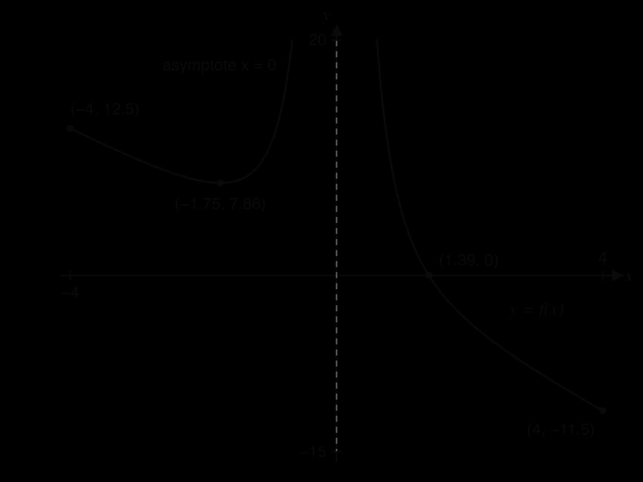
Sketch of y = 8/x² − 3x for −4 ≤ x ≤ 4 with axes from −15 to 20: end points (−4, 12.5) and (4, −11.5), local minimum (−1.75, 7.86), zero (1.39, 0), and the y-axis x = 0 as a vertical asymptote that neither branch touches. — A complete sketch transferred from a GDC: the end points, the local minimum, the zero and the asymptote are all labelled, and both branches rise towards x = 0 without touching it.

The sketch of $y = \frac{8}{x^2} - 3x$ shows every feature the GDC found, with coordinates to 3 significant figures: the left branch starts at $(-4, 12.5)$ , falls to a local minimum at $(-1.75, 7.86)$ and then climbs towards the asymptote; the right branch comes down from the asymptote, crosses the $x$ -axis at $(1.39, 0)$ and ends at $(4, -11.5)$ . There is no $y$ -intercept, because $f(0)$ does not exist.

Let $f(x) = \frac{8}{x^2} - 3x$ , for $-4 \le x \le 4$ , $x \ne 0$ .

(a) Write down the equation of the vertical asymptote of the graph of $f$ .

(b) Sketch the graph of $y = f(x)$ for $-4 \le x \le 4$ , labelling the local minimum point, the zero and the end points with their coordinates.

Show the solution

(a) The term $\frac{8}{x^2}$ is undefined at $x = 0$ and becomes very large as $x$ approaches 0, so the vertical asymptote is $x = 0$ (the $y$ -axis). It is written as an equation, not as "0".

(b) GDC working. Enter $Y_1 = 8/x^2 - 3x$ with window $-4 \le x \le 4$ , $-15 \le y \le 20$ . (A table shows $f(-4) = 12.5$ and $f(4) = -11.5$ , and values near $x = 0$ are large and positive, so this $y$ -range shows the whole curve.)

Minimum tool on the left branch: $x = -1.7471\ldots$ , $y = 7.8622\ldots$ , so the local minimum is $(-1.75, 7.86)$ .
Zero tool on the right branch: $x = 1.3867\ldots$ , so the zero is $(1.39, 0)$ .
End points from the table: $(-4, 12.5)$ and $(4, -11.5)$ .

Sketch. Draw axes labelled $x$ and $y$ , mark −4 and 4 on the $x$ -axis and −15 and 20 on the $y$ -axis, and draw the asymptote $x = 0$ as a dashed line (here it lies along the $y$ -axis). Plot the four labelled points and join them as in the figure: the left branch falls from $(-4, 12.5)$ to the minimum and then rises steeply beside the asymptote; the right branch descends from beside the asymptote through the zero to $(4, -11.5)$ . Neither branch touches $x = 0$ , and the curve does not continue past $x = -4$ or $x = 4$ .

Sketching a sinusoidal model over a given domain

Periodic functions are where a careless sketch most often has the wrong shape. A wind turbine has its hub 80 m above the ground and blades 35 m long, and turns once every 4 seconds. The height, in metres, of the tip of one blade $t$ seconds after it points straight down is modelled by

h(t) = 80 - 35\cos(90t°), \quad t \ge 0.

The tip is lowest, $80 - 35 = 45$ m, when the cosine is 1, and highest, $80 + 35 = 115$ m, when the cosine is −1. The cosine returns to the same value every time $90t$ increases by 360, so every 4 seconds. The parameters and their meanings belong to subtopic 2.5, Modelling with functions; graphing the model only needs these values.

Sketch the graph of $h(t) = 80 - 35\cos(90t°)$ for $0 \le t \le 8$ , clearly labelling the coordinates of the maximum and minimum points.

Show the solution

GDC working. Put the GDC in degree mode. Enter $Y_1 = 80 - 35\cos(90x)$ with window $0 \le x \le 8$ , $0 \le y \le 130$ .

Minimum tool: minima at $(0, 45)$ , $(4, 45)$ and $(8, 45)$ (the first and last are the end points of the domain).
Maximum tool: maxima at $(2, 115)$ and $(6, 115)$ .

Sketch. Label the axes $t$ (seconds) and $h$ (metres). Mark the five points and join them with a smooth, wave-shaped curve that:

starts at $(0, 45)$ and stops at $(8, 45)$ , not beyond;
is symmetrical about the line $h = 80$ , halfway between the maximum and minimum heights;
is rounded at the bottom (bending upwards near each minimum) and rounded at the top, not pointed.

h(t) = 80 − 35cos(90t°)

Two complete turns of the blade tip: the curve is symmetrical about h = 80 and rounded at every maximum and minimum.

In radian mode the same keystrokes would graph $80 - 35\cos(90t)$ with $90t$ in radians, a curve with period about 0.07 s, which looks like a solid block on the screen: a clear sign that the mode is wrong.

Sketching from information or a context

Some sketches start from words, not formulas. The description fixes the key features, and the context fixes the shape between them. The method is to list the facts, turn each into a point, a line or a direction on the axes, and then join them with the simplest smooth curve that agrees with all of them.

The temperature inside a car parked in strong sunshine gives an example. The temperature is 22 °C when the car is locked, rises quickly at first, then more and more slowly, and never exceeds 52 °C.

Three facts follow from this description. The graph starts at $(0, 22)$ . It rises throughout, steeply at first and then flattening. It approaches but stays below the line $T = 52$ , which is a horizontal asymptote, drawn dashed. A curve that rises in a straight line, or levels off at 52 and then stops, contradicts the description.

A ball is thrown upwards from the top of a cliff 20 m above the sea. It reaches a greatest height of 31.25 m above the sea after 1.5 seconds and lands in the sea after 4 seconds. Its height above the sea, $h$ metres, is a quadratic function of time, $t$ seconds.

Sketch the graph of $h$ against $t$ for the whole flight, labelling the key features.

Show the solution

List the facts and what each gives on the graph:

thrown from 20 m at $t = 0$ : the start point $(0, 20)$ , the $h$ -intercept;
greatest height 31.25 m at 1.5 s: the maximum point $(1.5, 31.25)$ ;
lands in the sea at 4 s: the end point $(4, 0)$ , on the $t$ -axis;
quadratic: a smooth curve shaped like an upside-down U, symmetrical about the vertical line $t = 1.5$ .

Draw axes labelled $t$ (s) and $h$ (m), mark the three points, and join them with a smooth curve that rises from $(0, 20)$ to a rounded top at $(1.5, 31.25)$ and falls more and more steeply to $(4, 0)$ . The curve stops at $t = 0$ and $t = 4$ : before the throw and after the splash, the formula no longer describes the ball.

As a check on the shape, the point mirroring $(0, 20)$ in the line $t = 1.5$ is $(3, 20)$ , so the ball is back at cliff height after 3 seconds and falls the last 20 m in 1 second.

Revision Village, “Sketching Functions with a Calculator”: although made for the Analysis and Approaches course, it shows the same routine of finding each key feature on the GDC and copying it, labelled, onto paper.

Sums and differences of functions

Two functions with the same input can be combined output by output. If a shop's income from sales and its income from delivery charges both depend on the number of orders, the total income is the sum of the two functions; the money left after costs is a difference.

Subtracting works in the same way, output by output, but the order of the two functions now matters.

The rule works point by point, which gives a way to build the graph of a sum by hand. At each input, the height of $f + g$ is the height of $f$ plus the height of $g$ , with signs: where $g$ is negative the sum lies below $f$ , and where $g$ is zero the graphs of $f$ and $f + g$ meet. For example, with $f(x) = x^2$ and $g(x) = 4 - 2x$ :

\begin{aligned} (f + g)(3) &= f(3) + g(3) = 9 + (-2) = 7 \\ (f - g)(3) &= f(3) - g(3) = 9 - (-2) = 11 \end{aligned}

Algebraically, $(f + g)(x) = x^2 - 2x + 4$ and $(f - g)(x) = x^2 + 2x - 4$ , and substituting $x = 3$ into these gives the same 7 and 11. The order matters for a difference: $(g - f)(3) = -11$ , the negative of $(f - g)(3)$ .

The domain of a sum or difference consists of the inputs where both functions are defined. If $f(x) = \sqrt{x}$ and $g(x) = \frac{1}{x - 2}$ , then $f + g$ needs $x \ge 0$ for the square root and $x \ne 2$ for the fraction, so its domain is the set of inputs that satisfy both conditions.

\text{domain of } f + g:\quad x \ge 0 \text{ and } x \ne 2

Graphing sums and differences on a GDC

A GDC builds the sum without any algebra. Store the two functions as $Y_1$ and $Y_2$ , then define $Y_3 = Y_1 + Y_2$ (or $Y_1 - Y_2$ ) by inserting the names $Y_1$ and $Y_2$ from the variables menu (VARS → Y-VARS → Function on a TI-84 Plus CE; on a Casio fx-CG50, VARS → GRAPH → Y followed by the function's number). This has two advantages over typing out the combined formula: there is no chance of an algebra or bracket error, and changing $Y_1$ or $Y_2$ updates $Y_3$ automatically.

Graphing all three together shows how the sum is built. The functions $Y_1$ and $Y_2$ can be hidden afterwards (de-selected) so that only $Y_3$ is drawn and the analysis tools act on it.

Revenue, cost and profit

The most common difference of functions in applied problems is profit. A business that sells $x$ items has a cost function $C(x)$ (subtopic 2.2) and earns money from the sales.

Revenue is not the same as profit, because the costs of making the items have not yet been paid out of it.

Graphing $R$ , $C$ and $P = R - C$ on the same axes links the three. The profit at any $x$ is the vertical gap between the revenue and cost graphs, positive where revenue is above cost. Where the two graphs cross, the gap is zero, so the profit graph crosses the horizontal axis at the same $x$ . Those values are the break-even points, studied as intersections in subtopic 2.4.

A bakery sells cupcakes for $3.50 each. Its weekly cost, in dollars, of making $x$ cupcakes is modelled by $C(x) = 120 + 1.2x + 0.002x^2$ , for $0 \le x \le 800$ .

(a) Write down the revenue function $R(x)$ .

(b) Show that the weekly profit is $P(x) = -0.002x^2 + 2.3x - 120$ .

(c) Use your GDC to sketch $R$ , $C$ and $P$ on the same axes for $0 \le x \le 800$ .

(d) Find the number of cupcakes the bakery must sell in a week to make a profit, and the greatest weekly profit.

Show the solution

(a) Each cupcake brings in $3.50, so $R(x) = 3.5x$ .

(b) Profit is revenue minus cost, with the whole cost in brackets:

\begin{aligned} P(x) &= R(x) - C(x) \\ &= 3.5x - (120 + 1.2x + 0.002x^2) \\ &= 3.5x - 120 - 1.2x - 0.002x^2 \\ &= -0.002x^2 + 2.3x - 120 \end{aligned}

(c) GDC working. $Y_1 = 3.5x$ , $Y_2 = 120 + 1.2x + 0.002x^2$ , $Y_3 = Y_1 - Y_2$ , window $0 \le x \le 800$ , $-200 \le y \le 2900$ .

R(x) = 3.5x
C(x)
P(x) = R(x) − C(x)

Profit is the vertical gap between revenue and cost: it is zero where the two graphs cross (x ≈ 54.8) and greatest at x = 575.

(d) The zero tool on $Y_3$ gives $x = 54.78\ldots$ ; profit is positive for larger $x$ . Because $x$ is a whole number of cupcakes, the bakery makes a profit when it sells at least 55 cupcakes a week. (The second zero, near $x = 1095$ , lies outside the domain.)

The maximum tool on $Y_3$ gives $(575, 541.25)$ : the greatest weekly profit is $541.25, when 575 cupcakes are sold.

The $P$ -intercept, $P(0) = -120$ , is the loss in a week with no sales: the fixed cost of $120.

Case study: the Keeling Curve as a sum of two functions

Since 1958, the concentration of carbon dioxide (CO₂) in the air has been measured continuously at Mauna Loa Observatory in Hawaii. The graph of the monthly averages, called the Keeling Curve after the scientist who began the record, rises year after year and also wobbles up and down within every year. The wobble is seasonal: the concentration is highest around May and lowest around September or October, because plants in the Northern Hemisphere, where most land is, take in CO₂ as they grow in spring and summer and release it as leaves decay in autumn and winter.

These two effects can be modelled separately and added. For the 24 months of 2024 and 2025, with $t$ the number of months after January 2024, fitting a straight line and a 12-month sine wave to the data together gives a long-term trend and a seasonal cycle (coefficients rounded):

T(t) = 423.2 + 0.244t, \qquad S(t) = 3\sin(30t°), \qquad C(t) = T(t) + S(t).

Here $C$ is the CO₂ concentration in parts per million (ppm). The trend rises by 0.244 ppm a month, about 2.9 ppm a year, and the cycle adds up to 3 ppm above the trend or takes up to 3 ppm below it, a swing of about 6 ppm each year. The graph of the seasonal part alone shows a wave that repeats every 12 months.

S(t) = 3sin(30t°)

The seasonal part alone: up to 3 ppm above the trend in spring and 3 ppm below it in autumn, repeating every 12 months.

On a GDC (in degree mode), the model is built exactly as a sum: $Y_1 = 423.2 + 0.244x$ , $Y_2 = 3\sin(30x)$ , $Y_3 = Y_1 + Y_2$ , with window $0 \le x \le 23$ , $418 \le y \le 433$ . The resulting graph rides along the trend line, rising above it in the first half of each year and dropping below it in the second half. Against the measured monthly averages, the sum follows the data closely.

Month	Jan 2024	Apr 2024	Jul 2024	Oct 2024	Jan 2025	Apr 2025	Jul 2025	Oct 2025
$t$	0	3	6	9	12	15	18	21
Measured CO₂ (ppm)	422.80	426.51	425.55	422.38	426.65	429.64	427.87	424.87
Model $C(t)$ (ppm)	423.20	426.93	424.66	422.40	426.13	429.86	427.59	425.32

Source: NOAA Global Monitoring Laboratory, Mauna Loa CO₂ monthly mean data (co2_mm_mlo), accessed October 2026.

trend T(t)
C(t) = T(t) + S(t)

The sum of a rising line and a 12-month wave follows the monthly Mauna Loa readings (points) to within about 1 ppm. Source: NOAA GML, 2026.

Every model value is within about 1 ppm of the measurement, against a seasonal swing of about 6 ppm, so the sum captures both effects. The table also shows the model's main weakness. The real cycle is lopsided: the concentration climbs slowly from October to May and falls quickly from June to September, while a sine curve rises and falls at the same rate. The model therefore peaks in April ( $t = 3$ and $t = 15$ ) rather than in May, and it is too high in spring and too low in early summer. A straight trend is also only right for a short period: over the whole record since 1958 the yearly increase has itself grown, so extending $T(t)$ decades into the past or future would be extrapolation beyond what the model can support.

Exam focus

Graphing appears in most function questions on Paper 2 and in many on Paper 1. The graph is rarely the whole question: a typical part asks you to sketch a function, often one not met before, worth 2 to 4 marks, followed by parts that use the graph to find a maximum, solve an equation or interpret the result in context. Draw appears when an accurate graph is needed on given axes or graph paper, often to add a line; plot appears with data. Sums and differences appear mainly as profit, revenue and cost, or as a total built from two parts.

What the markscheme rewards on a sketch:

the correct shape: rising and falling in the right places, the right curvature, smooth, with asymptotic behaviour that approaches but does not cross or veer away from the asymptote;
key points labelled with coordinates (or values marked on the axes): maximum, minimum, intercepts, and any point the question names;
the curve drawn in the given domain only;
axes labelled with the question's variables and some indication of scale.

The GDC is expected throughout. Write down the function you entered and, if it helps, the window; give coordinates found with the analysis tools to 3 significant figures, not values read with the trace cursor.

A small company makes and sells $x$ hundred phone cases a week. Its weekly revenue and cost, both in hundreds of dollars, are modelled by

R(x) = 40x - 2x^2, \qquad C(x) = 0.5x^3 - 4x^2 + 20x + 30, \qquad 0 \le x \le 9.

(a) Write down the value of $C(0)$ and interpret it in context. [2]

(b) Show that the weekly profit $P(x)$ , in hundreds of dollars, is given by $P(x) = -0.5x^3 + 2x^2 + 20x - 30$ . [2]

(c) Sketch the graph of $y = P(x)$ for $0 \le x \le 9$ , labelling the maximum point and the $x$ -intercepts with their coordinates. [4]

(d) Write down the number of phone cases the company should make each week to maximise its profit, and the maximum profit in dollars. [2]

(e) Find the range of weekly production, in hundreds of cases, for which the company makes a profit. [2]

Show the markscheme

(a) $C(0) = 30$ A1

The fixed weekly cost is $3000 (the cost when nothing is made). R1

(b) $P(x) = (40x - 2x^2) - (0.5x^3 - 4x^2 + 20x + 30)$ M1

$= 40x - 2x^2 - 0.5x^3 + 4x^2 - 20x - 30$ A1

$P(x) = -0.5x^3 + 2x^2 + 20x - 30$ AG

Note: the line with the brackets removed must be seen; substituting values to check the result earns no marks.

(c) Shape: smooth curve starting below the axis at $(0, -30)$ , rising to a single maximum, then falling below the axis to finish at $(9, -52.5)$ , drawn for $0 \le x \le 9$ only. A1

Maximum labelled $(5.22, 57.8)$ . A1

$x$ -intercepts labelled $(1.38, 0)$ and $(8.04, 0)$ . A1A1

(Unrounded values: maximum $(5.2206\ldots, 57.778\ldots)$ ; intercepts $1.3758\ldots$ and $8.0449\ldots$ .)

(d) 522 phone cases (accept 520) A1

maximum profit $= \$5780$ (accept $\$5777.85$ ) A1

(e) $P(x) > 0$ between the $x$ -intercepts (M1)

$1.38 < x < 8.04$ A1

Total [12]

Answers in context need care with units. Here $x$ is in hundreds of cases and $P$ in hundreds of dollars, so the GDC's 5.22 and 57.8 become 522 cases and $5780.

A common trap combines the window and the domain. The question restricts $x$ to $0 \le x \le 9$ , so the sketch must end at $(9, -52.5)$ ; a GDC left on its default window would show the cubic continuing beyond both ends.

Practice questions

The function $g$ is defined by $g(x) = x^3 - 5x + 2$ . Determine whether the point $(-2, 4)$ lies on the graph of $y = g(x)$ . [2]
Explain the difference between the command terms draw and sketch when applied to the graph of a function. [2]
A rectangular field has perimeter 200 m and width $x$ m. Its area is $A(x) = x(100 - x)$ . (a) Write down a suitable domain for $x$ . (b) Write down a suitable viewing window for graphing $A$ on a GDC. [3]
Let $f(x) = x + \frac{12}{x^2}$ , $x \ne 0$ . Sketch the graph of $y = f(x)$ for $-4 \le x \le 6$ , labelling the zero, the local minimum and the end points with their coordinates, and showing the vertical asymptote. [4]
Let $f(x) = 2x + 1$ and $g(x) = x^2 - 3$ . (a) Find $(f + g)(2)$ and $(f - g)(2)$ . (b) Write down an expression for $(f - g)(x)$ . [3]
A seat on a Ferris wheel has height $h(t) = 50 - 45\cos(6t°)$ metres, $t$ seconds after the ride starts. Sketch the graph of $h$ for $0 \le t \le 90$ , labelling the maximum and minimum points. [3]
A theatre sells tickets for $18 each. The cost of putting on a show for $x$ people is $C(x) = 2400 + 4x$ dollars, for $0 \le x \le 450$ . (a) Write down the revenue function. (b) Find the profit function. (c) Find the smallest number of tickets that must be sold to make a profit. [5]
A cup of coffee is poured at 85 °C into a room at 20 °C. It cools quickly at first and then more slowly, getting closer and closer to room temperature. Sketch a graph of its temperature against time, labelling the key features. [3]
A function is given by $V(x) = 0.02x^3 - 1.2x^2 + 18x$ , $0 \le x \le 42$ . (a) Find the coordinates of the local maximum and local minimum points. (b) Write down the greatest value of $V$ on the domain, and explain why it is not at the local maximum. [5]

Answers

$g(-2) = -8 + 10 + 2 = 4$ , so yes, $(-2, 4)$ lies on the graph.
A drawing is accurate and to scale, with points plotted correctly and joined by a ruled line or smooth curve; a sketch shows the general shape and the relevant features, labelled, but need not be to scale.
(a) $0 < x < 100$ (width and length both positive). (b) For example $0 \le x \le 100$ , $0 \le y \le 3000$ ; the largest area is $A(50) = 2500$ .
GDC: $Y_1 = x + 12/x^2$ , window $-4 \le x \le 6$ , $-6 \le y \le 20$ . Zero $(-2.29, 0)$ ( $-2.2894\ldots$ ); local minimum $(2.88, 4.33)$ ( $2.8845\ldots, 4.3267\ldots$ ); end points $(-4, -3.25)$ and $(6, 6.33)$ ( $6.3333\ldots$ ); vertical asymptote $x = 0$ , both branches rising towards it.
(a) $f(2) = 5$ , $g(2) = 1$ ; $(f + g)(2) = 6$ , $(f - g)(2) = 4$ . (b) $(f - g)(x) = 2x + 1 - (x^2 - 3) = -x^2 + 2x + 4$ .
Degree mode; minimum points $(0, 5)$ and $(60, 5)$ ; maximum points $(30, 95)$ and $(90, 95)$ , the second also the end point. Symmetrical about $h = 50$ , period 60 s, drawn only for $0 \le t \le 90$ .
(a) $R(x) = 18x$ . (b) $P(x) = 18x - (2400 + 4x) = 14x - 2400$ . (c) $P(x) = 0$ at $x = 171.43\ldots$ ; profit needs at least 172 tickets.
Start at $(0, 85)$ ; decreasing curve, steep at first then flattening; dashed horizontal asymptote $T = 20$ , approached from above but never reached; axes labelled time and temperature (°C).
(a) GDC maximum $(10, 80)$ , minimum $(30, 0)$ ( $V(30) = 540 - 1080 + 540 = 0$ ). (b) $V(42) = 1481.76 - 2116.8 + 756 = 120.96$ , so the greatest value is 121 (120.96), at the end point $x = 42$ . After the local minimum the curve rises again and passes the local maximum value of 80 before the domain ends, so the end point must be checked as well as the turning points.

Summary

The graph of a function is the set of points $(x, f(x))$ ; a point $(a, b)$ lies on $y = f(x)$ exactly when $f(a) = b$ .
A table of values gives exact points to plot; points from a continuous function are joined by a smooth curve, points from a discrete domain are left unjoined.
The viewing window decides what part of the graph is seen: set $x$ to the domain, choose $y$ from the table or by automatic scaling, and zoom out to check nothing is hidden.
Read features with the GDC's analysis tools (value, zero, maximum, minimum, intersection), not the trace cursor; use degree mode for trigonometric models.
Plot marks points; sketch gives the shape with labelled key features, not to scale; draw gives an accurate graph to scale.
Transferring a graph to paper: set the window, find every key feature, label the axes with the question's variables, mark the features, join them smoothly, respect asymptotes, and stop at the end points.
A sketch from words turns each fact into a point, line or direction, then joins them with the simplest smooth curve that agrees with all of them.
$(f + g)(x) = f(x) + g(x)$ and $(f - g)(x) = f(x) - g(x)$ ; on a GDC use $Y_3 = Y_1 + Y_2$ or $Y_1 - Y_2$ .
Profit = revenue − cost, $P(x) = R(x) - C(x)$ ; the profit graph is zero where the revenue and cost graphs cross.

Self-check

To do:
I can test whether a point lies on a graph by substituting into $y = f(x)$ .
To do:
I can make a table of values and use it to plot points.
To do:
I can decide whether plotted points should be joined by a smooth curve.
To do:
I can enter a function with fractions, powers and negative signs correctly, using brackets.
To do:
I can choose a viewing window from a domain and a context, and change it when features are hidden.
To do:
I can set my GDC to degree mode before graphing a trigonometric model.
To do:
I can find coordinates with the analysis tools rather than the trace cursor.
To do:
I can explain the difference between plot, sketch and draw.
To do:
I can draw an accurate graph with a suitable scale on each axis.
To do:
I can transfer a GDC graph to paper with labelled axes, coordinates, asymptotes and end points.
To do:
I can sketch a graph from a description in words.
To do:
I can calculate $(f + g)(x)$ and $(f - g)(x)$ for a given $x$ and graph them with $Y_3 = Y_1 \pm Y_2$ .
To do:
I can write a profit function from revenue and cost, using brackets correctly.
To do:
I can interpret the zeros and the maximum of a profit graph in context.

Questions on 2.3

33 exam-style questions on this subtopic, written in the style of the IB papers. The first has its markscheme open. Counted on 20 October 2026

Question 1 · AI-002546 marks

A museum opens a new dinosaur exhibition. The number of visitors to the exhibition, $N$ thousand per week, $t$ weeks after it opens, can be modelled by

N(t) = 12t\,\mathrm{e}^{-0.4t}, \quad 0 \le t \le 12.

(a)
Sketch the graph of $N$ for $0 \le t \le 12$ , labelling the maximum point with its coordinates.
3 marks
Markscheme (a)
A1 for a curve starting at the origin, increasing to a single maximum, then decreasing towards (but not reaching) the $t$ -axis
A1 for the maximum point labelled $(2.5,\ 11.0)$ $(11.0363\ldots)$
A1 for the curve drawn only for $0 \le t \le 12$ , ending at approximately $(12,\ 1.19)$ , above the $t$ -axis
Note: Award the second mark for the maximum within half a grid square if coordinates are not written, provided the scale is shown.
[3 marks]
(b)
Write down the greatest number of visitors in one week, according to the model.
1 mark
Markscheme (b)
$11\,000$ visitors (accept $11\,036$ ) A1
Note: Accept $11.0$ thousand. Do not accept $11$ alone without reference to thousands.
[1 mark]
(c)
Find the values of $t$ for which there are $10\,000$ visitors per week.
2 marks
Markscheme (c)
sketch of $N$ with the line $N = 10$ OR $12t\,\mathrm{e}^{-0.4t} = 10$ (M1)
$t = 1.55$ and $t = 3.78$ $(1.54765\ldots,\ 3.78033\ldots)$ A1
Note: Award A1 only if both values are given.
[2 marks]

Question 2 · AI-002556 marks

Femi is investigating how bright a lamp appears at different distances. The intensity of the light, $I$ lux, at a distance of $d$ metres from the lamp is given by $I = \dfrac{36}{d^2}$ , for $d > 0$ .

The following table shows some values of $I$ .

$d$ (m)	1	1.5	2	3	4	5	6
$I$ (lux)	36	$p$	9	$q$	2.25	1.44	1

(a)
Find the value of $p$ and the value of $q$ .
2 marks
(b)
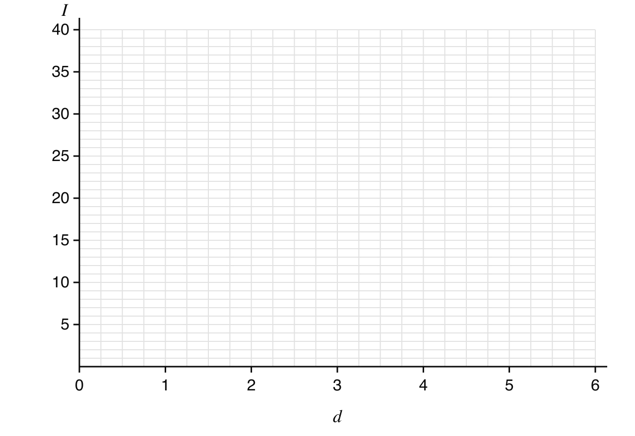
On the following grid, draw the graph of $I = \dfrac{36}{d^2}$ for $1 \le d \le 6$ .
3 marks
(c)
Use your graph to estimate the distance from the lamp at which the intensity is 6 lux.
1 mark

Answer it, then compare with the markscheme.Check this one with a free account

Question 3 · AI-002566 marks

Hannah pours a cup of tea at $85\,°\mathrm{C}$ and leaves it on her desk in a room kept at a constant $21\,°\mathrm{C}$ . The tea cools quickly at first and then more and more slowly, getting closer and closer to the temperature of the room.

Let $T$ be the temperature of the tea, in $°\mathrm{C}$ , $t$ minutes after it was poured.

(a)
Sketch a graph of $T$ against $t$ for $0 \le t \le 60$ . Label clearly the value where the graph meets the $T$ -axis and the equation of any asymptote.
3 marks
(b)
The temperature of the tea can be modelled by $T(t) = 21 + 64\,\mathrm{e}^{-0.08t}$ .
Find the time it takes for the tea to cool to $40\,°\mathrm{C}$ .
2 marks
(c)
Hannah claims that, according to the model, the tea will eventually cool to $20\,°\mathrm{C}$ . Explain why she is wrong.
1 mark

Answer it, then compare with the markscheme.Check this one with a free account

Key terms introduced here

Notes on 2.3 Graphing functions with technology

Learning objectives

Introduction

The graph of a function and its equation

Tables of values

Plotting points and joining them

Graphing with technology

Entering a function

The viewing window

Choosing a window from the context

Reading values from the graph

Functions not met elsewhere

Key features

Draw, sketch and plot

Drawing a graph accurately

Transferring a graph from screen to paper

A routine for transferring a graph

Sketching a sinusoidal model over a given domain

Sketching from information or a context

Sums and differences of functions

Graphing sums and differences on a GDC

Revenue, cost and profit

Case study: the Keeling Curve as a sum of two functions

Exam focus

Practice questions

Summary

Self-check

Questions on 2.3

Markscheme (a)

Markscheme (b)

Markscheme (c)

Carry on with 2.3 in Augment