2.10 Scaling very large and small numbers using logarithms

Learning objectives

• Explain why a logarithmic scale suits data that span several orders of magnitude or where the rate of growth matters more than the absolute size.

• Read values from a logarithmic axis, including between the labelled powers of 10.

• Show that an exponential relationship $y = ab^x$ or $y = a\mathrm{e}^{kx}$ gives a straight line when $\ln y$ is plotted against $x$.

• Show that a power relationship $y = ax^n$ gives a straight line when $\ln y$ is plotted against $\ln x$.

• Determine whether data have an exponential or a power relationship by linearizing them and comparing the straight-line fits.

• Find the parameters of an exponential or power model from the gradient and intercept of a best-fit line on transformed data, using technology.

• Interpret given semi-log and log-log graphs, including gradients, intercepts and the meaning of a straight line.

• Use the equation of a line on transformed axes to make predictions, writing it in the variables of the context.

Introduction

Many quantities in science, economics and technology range over enormous spans. The number of transistors on a computer chip rose from a few thousand in 1971 to billions forty years later; the intensity of sounds that the human ear can detect varies by a factor of more than a million million; the planets of the solar system take from under three months to over 160 years to orbit the Sun. On an ordinary graph, data like these squash almost every point into one corner. Logarithms solve the problem by turning multiplication into addition: on a logarithmic axis, every factor of 10 takes up the same distance.

Logarithms also straighten curved relationships. Taking logarithms turns exponential and power relationships into straight lines, and straight lines are easy to recognise, to fit and to read. This idea, called linearization, gives a reliable way to decide which kind of model suits a set of data and to find its parameters from a gradient and an intercept.

Scaling with logarithms

Why a linear scale fails

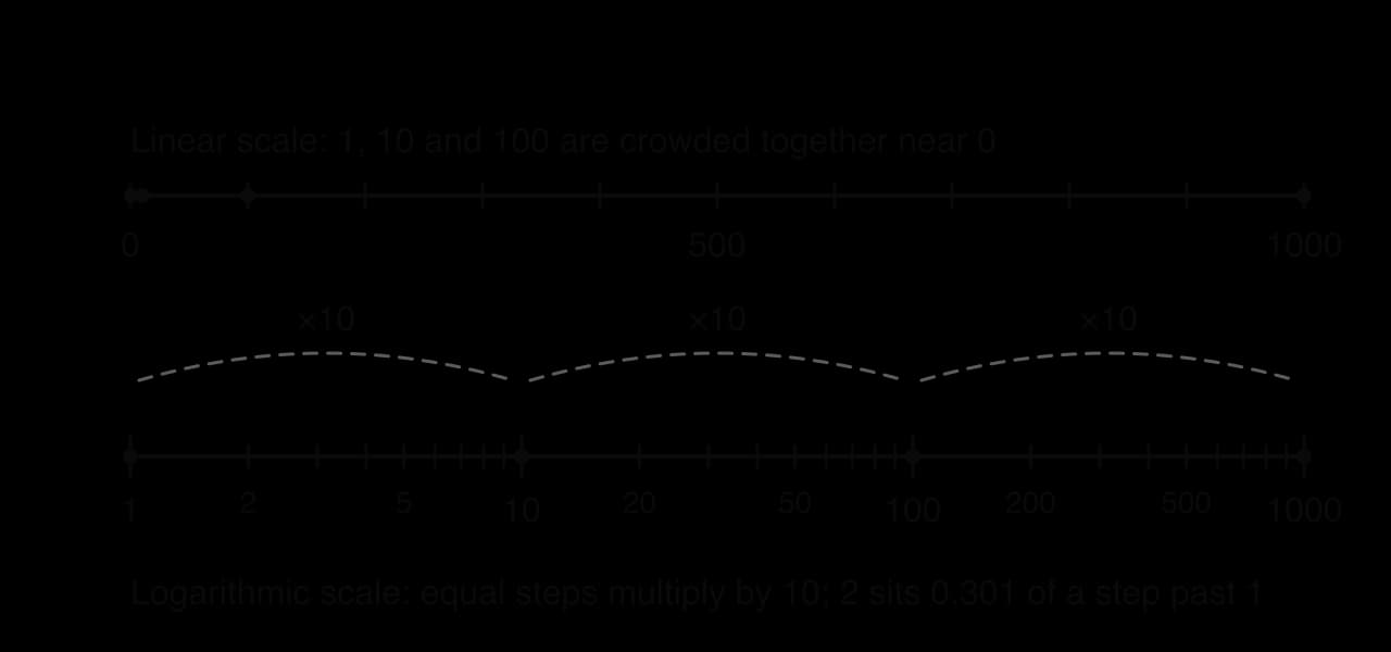
On an ordinary (linear) axis, equal distances represent equal differences: the gap from 0 to 100 is the same length as the gap from 900 to 1000. For data spanning several orders of magnitude, this wastes almost the whole axis on the largest values. If an axis must reach 1000, the values 1, 10 and 100 all crowd into the first tenth of it, and differences between them cannot be seen.

A logarithmic scale spaces values by their logarithms instead. The position of a value $v$ on a base-10 log axis is $\log v$, so the values 1, 10, 100 and 1000 sit at positions 0, 1, 2 and 3, equally spaced. Equal distances represent equal ratios, and each step of one unit multiplies the value by 10.

Reading a logarithmic axis

The labelled gridlines on a log axis are usually powers of 10, sometimes written $10^0, 10^1, 10^2, \ldots$ and sometimes as 1, 10, 100. The unlabelled minor gridlines between two powers of 10 stand for 2, 3, …, 9 times the lower power. They are not equally spaced: the gridline for 2 sits $\log 2 \approx 0.301$

To read a value at a point on a log axis, measure what fraction $p$ of the way the point lies from one power of 10 to the next. If the point is a fraction $p$ of the way from $10^m$ to $10^{m+1}$, its position is $m + p$

A point 0.6 of the way from 100 to 1000 is at position 2.6, so its value is $10^{2.6} \approx 398$, not 640. The reverse conversion uses the logarithm: the value 300 is at position $\log 300 = 2.477$, nearly half-way between 100 and 1000.

Familiar logarithmic scales

Several standard measurement scales are logarithmic, because the quantities they describe range over many orders of magnitude. Subtopic 1.5, Exponents and introduction to logarithms, introduces them; here they illustrate why the scaling is chosen.

• Acidity. The pH of a solution is $-\log[\mathrm{H}^+]$. Hydrogen-ion concentrations from about 1 to $10^{-14}$ mol per litre become a compact scale from 0 to 14, and each step of 1 in pH is a factor of 10 in concentration.

• Sound. The decibel level of a sound of intensity $I$ watts per square metre is $L = 10\log\left(\frac{I}{I_0}\right)$

When to choose a logarithmic scale

A logarithmic scale is the right choice in two situations. The first is when the data span several orders of magnitude, so that a linear scale would hide most of the values: country populations from thousands to over a billion, or earthquake amplitudes. The second is when the rate of growth matters more than the absolute size. On a log scale, a constant percentage growth rate appears as a straight line, so a steeper line means faster percentage growth, whatever the size of the quantity.

The second reason explains why charts of a spreading epidemic, a company's users or the price of a share over a century are often drawn on a logarithmic axis. On a linear axis the latest growth always looks most alarming, because the absolute increases are largest; on a log axis, a straight stretch shows a steady rate of growth, a steepening line shows the rate increasing, and a flattening line shows growth slowing. The Gapminder Foundation's charts of life expectancy against income per person use a logarithmic income axis, so that countries with incomes of a few hundred dollars and those with incomes of tens of thousands can be compared on one chart, and equal distances represent equal percentage differences in income.

YouTube

Semi-log graphs and exponential relationships

Taking logarithms of an exponential

An exponential relationship $y = ab^x$ multiplies $y$ by the constant factor $b$ each time $x$ increases by 1. Taking natural logarithms of both sides and using the product and power laws of logarithms (subtopic 1.9) gives

The last line has the form $Y = mX + c$ with $Y = \ln y$ and $X = x$. So the graph of $\ln y$

A semi-log graph can be drawn in two equivalent ways. Either the values of $y$ are plotted on an axis with a logarithmic scale (labelled 1, 10, 100, …), or the numbers $\ln y$ are calculated and plotted on an ordinary axis. The shapes are identical; only the labels differ.

To recover the model from a straight line on a semi-log graph, undo the logarithms:

With base-10 logarithms, $b = 10^m$ and $a = 10^c$. In both cases the model can also be written directly from the line: $\ln y = mx + c$

From two points on the line

When two points on the straight line of a semi-log graph are known, the method is the straight-line work of subtopic 2.1, Equations of straight lines, in the transformed variables.

Doubling time from a semi-log graph

On a semi-log graph with base-10 logarithms, a straight line $\log y = mx + c$ means $y$ is multiplied by $10^m$ each time $x$

A steeper line means a shorter doubling time. Lines with the same gradient on a semi-log graph describe quantities growing at the same percentage rate, even if one is a thousand times larger than the other.

Case study: Moore's law

In 1965 Gordon Moore, who later co-founded Intel, predicted that the number of components on an integrated circuit would double every year; in 1975 he revised the prediction to a doubling every two years. The prediction, known as Moore's law, held closely for decades, although the pace has slowed since around 2010. The transistor counts of a selection of Intel processors test it.

Source: Wikipedia, "Transistor count", microprocessor table, retrieved 2026.

On a linear axis these counts cannot be compared, because the first six processors would all sit on the horizontal axis next to the 2.3 billion of 2010. With $t$ as years after 1970 and $N$ as the number of transistors, the values of $\log N$ are easy to plot.

Linear regression of $\log N$ on $t$ with the GDC gives $\log N = 0.1496t + 3.191$, with Pearson's correlation coefficient $r = 0.999$

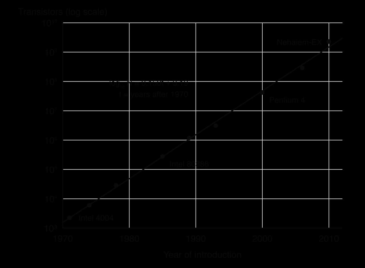
The parameters of the model follow from the gradient and intercept:

The transistor count grew by about 41% a year, doubling about every two years, in line with Moore's 1975 revision. The model can then be tested by extrapolation. For 2020 ($t = 50$) it predicts $10^{0.1496 \times 50 + 3.191} \approx 4.7 \times 10^{10}$ transistors. Apple's M1 processor, released in 2020, has about

Log-log graphs and power relationships

Taking logarithms of a power law

In a power relationship the variable is the base and the exponent is a constant.

Taking logarithms of both sides of $y = ax^n$:

This time the straight line appears when $\ln y$ is plotted against $\ln x$: both variables must be transformed. The gradient is the power $n$ and the intercept is $\ln a$.

The intercept on a log-log graph is the value of $\ln y$ where $\ln x = 0$, that is, where $x = 1$. This matches the power law, since $y = a \times 1^n = a$

What the gradient of a log-log graph means

The gradient $n$ of a log-log graph says how $y$ responds to proportional changes in $x$. Doubling $x$ multiplies $y$ by $2^n$

A straight line on a log-log graph means a power law. Only a line of gradient 1 corresponds to direct proportion $y = ax$; any other gradient describes a curve on ordinary axes.

Kepler's third law

Johannes Kepler published in 1619 the result that the square of a planet's orbital period is proportional to the cube of its average distance from the Sun (the semi-major axis of its orbit). In symbols, $T^2 \propto a^3$, or $T = ka^{1.5}$. The data of all eight planets give a striking log-log graph.

Source: NASA JPL Solar System Dynamics, "Planetary Physical Parameters" (sidereal orbital periods) and "Approximate Positions of the Planets" (semi-major axes, J2000), retrieved 2026. AU = astronomical unit.

Linear regression of $\ln T$ on $\ln a$ gives $\ln T = 1.4997\ln a + 0.0003$, with $r = 1.000$

The units chosen make the intercept zero: Earth has $a = 1$ and $T = 1$, so it sits at the origin of the log-log graph. With other units (kilometres and days), the gradient would still be 1.5, because changing units multiplies $a$ or $T$ by a constant, which shifts the line up or down without changing its gradient.

Linearizing data to choose a model

The idea of linearization

Curved data on an ordinary graph could follow many kinds of model, and the eye is poor at telling an exponential curve from a power curve. A straight line, though, is easy to judge. Transforming the variables with logarithms, and testing which transformation makes the data straight, gives the choice of model a clear test.

The two transformations to test are summarised in one table.

The rule to remember is that the variable that sits in a power gets logged together with $y$. In an exponential, $x$ is the exponent, so it stays as it is; in a power law, $x$ is the base, so it must be logged as well.

The method with technology

The GDC does the transforming and the fitting. The steps are the same for both models.

1. Enter the data: $x$ in list L1 and $y$ in list L2.

2. Create the transformed lists: L3 = ln(L2) and, for a power law, L4 = ln(L1).

3. Run linear regression of L3 on L1 (exponential test) and of L3 on L4 (power test). Record the gradient, the intercept and Pearson's correlation coefficient $r$ for each. On a TI-84 Plus CE the linear regression is under STAT → CALC (with MODE → STAT DIAGNOSTICS ON so that $r$ is shown); on a Casio fx-CG50 it is MENU → Statistics → CALC → REG → X → ax+b.

4. Choose the model whose transformed data are closer to a straight line: $r$

The value of $r$ on transformed data measures how close the transformed points are to a straight line, as in subtopic 4.4, Correlation and regression. A value of $r$ very close to 1 does not prove the model is right, but comparing the two values of $r$ for the same data is a fair way to choose between the two families, especially when combined with a look at the transformed points. Subtopic 4.13, Non-linear regression, fits the same models directly with the GDC's exponential and power regression; the parameters can differ slightly from those found by linearization, because the two methods minimise different errors.

A new website records its daily visits for its first six days (hypothetical data). Growth like this could be exponential or a power law, and the two linearizations decide between them.

A student drops a marble into a tray of fine sand from six heights and measures the diameter of each crater (hypothetical measurements). The diameter grows more and more slowly as the height increases, a shape that could be either a power law with a small power or a slowing exponential.

The crater example shows the value of linearization beyond curve fitting. A gradient of about 0.25 on the log-log graph means that doubling the drop height multiplies the crater diameter by only $2^{0.25} \approx 1.19$, and a sixteenfold increase in height is needed to double the diameter. A power this close to a simple fraction suggests a physical law behind the data, which a scientist would then try to explain.

Other linearizations

Logarithms of $x$ and $y$ are not the only way to straighten data, and other models need other transformations. The principle is always the same: rewrite the model so that it has the form $Y = mX + c$, and identify which expressions play the roles of $Y$ and $X$

• A natural logarithmic model $y = a + b\ln x$ is linear in $\ln x$: plot $y$ against $\ln x$.

• A rate model $k = A\mathrm{e}^{-c/T}$

The rate constant of a chemical reaction is measured at five temperatures (hypothetical data).

Interpreting semi-log and log-log graphs

Reading given graphs

Scientific reports and news articles often show a semi-log or log-log graph, or give the equation of its straight line. Reading one always uses the same three facts.

1. The type of graph identifies the model. A straight semi-log graph ($\log y$ against $x$) means exponential; a straight log-log graph ($\log y$ against $\log x$) means a power law.

2. The gradient is a rate or a power. On a semi-log graph the gradient is $\log b$

A graph that is straight in sections and then bends shows a change of behaviour: on a semi-log graph of cumulative cases in an epidemic, a straight early stretch shows exponential spread, and a later flattening shows the percentage growth rate falling.

The form $\log N = a - bM$ is the Gutenberg–Richter law of seismology; the values of $a$ and $b$ differ from region to region.

Interpreting gradients in context

The gradient of a straight line on transformed axes has a meaning that should be stated in the context's language, not just as a number.

• On a semi-log graph with natural logarithms, a gradient of $k$ means the quantity grows (or decays) by a factor $\mathrm{e}^{k}$ per unit of $x$; for small $k$, this is approximately a growth of $100k\%$

YouTube

Exam focus

Logarithmic scaling and linearization appear on HL Paper 1 as short questions of 4 to 7 marks, on Paper 2 as part of a longer modelling question, and on Paper 3, where a context often begins with linear regression and develops into an exponential or power model found by transforming the data. The command terms are show that (taking logarithms of a model), find (gradient, intercept and parameters), write down (the equation of a regression line from the GDC), hence (convert the line back to the model), explain or justify (why a straight graph supports a model) and interpret (a gradient in context). You will not be asked to draw or sketch a semi-log or log-log graph, but you must read them.

Recurring question shapes:

• A straight line through two given points on a graph of $\ln y$ against $x$ or $\ln y$ against $\ln x$: find the line, then the model, then a prediction.

• A table of data: find the regression line of the transformed variables with the GDC, then the parameters.

• "Show that $\ln y = \ldots$

What to write down: the linearized equation in the question's variables, the gradient calculation or the regression used (which variable on which), the conversion $a = \mathrm{e}^{\ldots}$ or $10^{\ldots}$, and the final model with its variables. Give answers in standard form, never calculator notation such as 4.7E10.

The full exam-style question uses a table of flow measurements over a V-shaped notch in a weir (hypothetical data).

When a question gives two points on a transformed line, the gradient is the first method mark and the conversion of the intercept with $\mathrm{e}$ or 10 is the last accuracy mark. Many candidates find the line correctly and then report the intercept itself as the parameter.

Answers involving parameters such as $k = 4.15 \times 10^{7}$ must be written in standard form. Calculator notation (4.15E7) is not accepted.

Practice questions

1. On a logarithmic axis, the labelled gridlines are 1, 10, 100 and 1000, equally spaced. A point lies 0.4 of the way from 10 to 100. Find the value it represents. [2]

2. The pH of a solution is $-\log[\mathrm{H}^+]$. Find the pH of a solution with $[\mathrm{H}^+] = 4.0 \times 10^{-9}$

Summary

• On a logarithmic scale, equal distances represent equal ratios; a value at position $m + p$ on a base-10 log axis is $10^{m + p}$. Log scales suit data spanning many orders of magnitude and graphs where the rate of growth matters.

• pH, decibels and the Richter scale are logarithmic scales: each unit (or 10 dB) is a factor of 10.

• An exponential $y = ab^x$

Self-check

• To do:

  I can explain when a logarithmic scale is better than a linear one.

• To do:

  I can read a value between gridlines on a logarithmic axis.

• To do:

  I can find the ratio of two values from their distance apart on a logarithmic axis, and explain why pH, decibels and earthquake magnitudes use logarithmic scales.

• To do:

  I can show that $y = ab^x$ gives a straight line of $\ln y$ against $x$