2.6 The modelling process

The modelling cycle

Modelling starts from a genuine problem: a question someone wants answered or a decision someone has to make. The real situation is always more complicated than any function, so the modeller simplifies it, writes down a model, and then checks whether the model behaves like the real thing. When it does not, the modeller changes something and tries again. This loop is called the modelling cycle.

The diagram of the cycle shows six stages arranged in a loop. The dashed arrow is the step that makes modelling a cycle rather than a list: when testing shows the model is not good enough, the modeller returns to the assumptions or the choice of function.

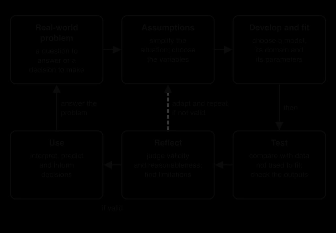
The stages group into three phases.

1. Develop and fit the model. Decide which quantities matter, state the assumptions, choose a type of function, decide a reasonable domain and find the parameters.

2. Test and reflect on the model. Compare the model's outputs with data that were not used to build it, check that its outputs are sensible, and judge how appropriate it is. If it fails, adapt it and go round again.

3. Use the model. Read values from it, interpret its parameters, make predictions and use the results to answer the original question.

Critical reflection is not confined to one stage. A modeller who finds a parameter with the wrong sign, or a domain that includes impossible values, reflects and adapts there and then, without waiting for a formal test.

Assumptions

Real situations involve far more influences than a function can hold. A modeller of a falling ball might ignore air resistance; a modeller of a town's population might ignore migration. Each such decision is an assumption.

Assumptions do three jobs. They decide which variables are included (time, but not temperature), they decide the type of relationship (a constant rate of change, a constant percentage change, a repeating pattern), and they set the conditions under which the model can be trusted. That last job matters most when the model is used, because a prediction made where an assumption no longer holds is unreliable.

There is always a balance between simplicity and accuracy. A model with few assumptions and many parameters can match the data closely but is hard to fit and interpret; a very simple model is easy to use but may miss important behaviour. A good modeller chooses the simplest model that answers the question to the accuracy needed.

Developing the model: choosing a type of function

Subtopic 2.5 gives a family of functions for each common pattern of change. Choosing between them uses three kinds of evidence: the context (what is known about how the quantity behaves), the shape of the data (how the values change from one step to the next), and the properties of the curve (intercepts, turning points, asymptotes, periodicity). A strong justification uses at least two of these.

Evidence from the context

Some contexts point straight to a family because of the mechanism behind them. A quantity that changes by the same amount in each time step suggests a linear model; one that changes by the same percentage suggests exponential growth or exponential decay; one that repeats every day or year suggests a sinusoidal model. A projectile under gravity follows a quadratic model, and a quantity proportional to a power of another follows direct variation or inverse variation.

Evidence from the shape of the data

When data are given at equally spaced inputs, simple arithmetic on the outputs shows the pattern of change. Subtracting each value from the next gives the first differences; subtracting those gives the second differences; dividing each value by the one before gives the ratios.

• Constant first differences mean the same amount is added each step: a linear model.

• Constant second differences (but changing first differences) mean a quadratic model. For $f(x) = ax^2 + bx + c$ with a step of 1, the first differences are $f(x+1) - f(x) = 2ax + a + b$, which go up by $2a$ each step, so the second differences are the constant $2a$.

• Constant ratios mean each value is the previous one multiplied by the same number: an exponential model with $c = 0$. For $f(x) = ka^x$, $\frac{f(x+1)}{f(x)} = \frac{ka^{x+1}}{ka^x} = a$

Real data never give exactly constant differences or ratios, because of measurement error and natural variation. "Approximately constant" is the test, and a scatter diagram drawn with technology is the quickest way to see the overall shape.

The table gives two quantities, $P$ and $Q$, measured at equal time intervals.

The graph of the data for $Q$ with two candidate models shows why the shape matters. A straight line through the first and last points misses every point in between, while the exponential curve passes through them all.

Evidence from the properties of the curve

The features of a graph, read with technology as in subtopic 2.4, Key features of graphs, also separate the families. A quadratic has exactly one turning point and is symmetrical about it. A cubic can have two turning points and up to three zeros. An exponential model $ka^x + c$ has no turning points and a horizontal asymptote $y = c$. An inverse variation $ax^{-n}$ has both axes as asymptotes. A sinusoidal model repeats with a fixed period and stays between a maximum and a minimum.

Predicting the parameters from the context

Before any calculation, the context often fixes the sign or approximate size of each parameter. Predicting them is a quick check on the fitting that follows: a fitted value with the wrong sign means an error in the working or a poor choice of model.

• The height of a thrown ball is a quadratic $at^2 + bt + c$ with $a < 0$ (the graph opens downwards), $b > 0$ (it starts by rising) and $c$ equal to the launch height. In metres and seconds, $a$ is close to $-4.9$, half the acceleration due to gravity.

• The temperature of a cooling drink is $ka^t + c$ with $0 < a < 1$ (decay), $c$ equal to the room temperature (the asymptote) and $k + c$

• The value of a car losing 15% a year is $k \times 0.85^t$, with $k$ the price when new.

• The daylight hours of a city are $a\cos(bt) + d$ with $d$ near 12 (the average day length over a year) and period 12 months, so $b = 360° \div 12 = 30°$.

Fitting the model: finding the parameters

Once a family is chosen, the parameters have to be given values that make the model match the situation. This is fitting the model.

Each unknown parameter needs one independent piece of information. A model with two unknown parameters needs two facts (two points, or one point and an asymptote), a model with three needs three, and so on. The table lists what fixes each model of subtopic 2.5.

The information comes in three main forms: initial conditions, features of the graph, and points that are substituted to give equations.

From initial conditions

An initial condition is the value of the model when the input is zero, usually at the start of the time period. Substituting $t = 0$ removes every term that contains $t$: for $ka^t$ it gives $k$, for $ka^t + c$ it gives $k + c$, and for a polynomial it gives the constant term. One parameter is then found with no simultaneous equations.

From features of the graph or the context

Some parameters are features of the graph and can be read off directly. For a sinusoidal model, the amplitude is half the distance from maximum to minimum, the principal axis lies halfway between them, and the period gives $b$:

For an exponential model $ka^x + c$, the constant $c$ is the horizontal asymptote, the value the quantity settles towards, which often comes from the context (room temperature, a machine's top speed, a minimum population). For a quadratic, the vertex lies on the axis of symmetry $x = -\frac{b}{2a}$, so a known vertex gives an equation linking $a$ and $b$.

By substituting points and solving equations with technology

When the model has several unknown parameters and no feature gives one directly, each known point is substituted into the general form. Every point gives one linear equation in the parameters, because the parameters appear only to the first power once numbers replace $x$ and $y$. Three points give a system of three linear equations, which the GDC solves directly.

The method for a quadratic $y = ax^2 + bx + c$ through three points:

1. Substitute each point $(x_i, y_i)$ to get $y_i = ax_i^2 + bx_i + c$, and simplify the numbers (square each $x_i$).

2. Write the three equations with $a$, $b$, $c$ in the same order in each, which is the layout the GDC's simultaneous equation solver uses.

3. Enter the coefficients in the solver (on a TI-84 Plus CE, the PlySmlt2 app's simultaneous equation solver; on a Casio fx-CG50, MENU → Equation → SIMUL), with 3 unknowns.

4. Write down the three equations and the solution, with each value labelled.

A cubic $y = ax^3 + bx^2 + cx + d$ needs four points. The $y$-intercept gives $d$ at once, which leaves three equations in $a$, $b$ and $c$, the most the method ever needs at SL.

Reasonable domain

A function written as a formula accepts any input, but a model only makes sense for some of them. Time before the start of an experiment, a negative number of items or a height below the ground are outside the situation being modelled. The domain of a model must therefore be chosen from the context, not taken as all real numbers.

Four considerations set the limits of a reasonable domain:

• The start of the situation. Usually $t \ge 0$, the start of the observation.

• The end of the situation. The ball lands, the tank empties, the ride finishes, the battery runs out. Solving "model $=$ boundary value" with technology gives the end point.

• The possible values. Numbers of people or items are whole numbers, so the domain is a set of integers and the graph is a set of points.

• The range of the data. Inside the range of the data the model has been checked; beyond it, the model has not.

The graph of Ayesha's ball model shows the reasonable domain as the solid part of the curve. Outside it the formula still produces numbers, including negative heights, but they describe nothing real.

Testing and reflecting on the model

A model that has been fitted to some information has not yet been shown to be any good. It agrees with the points used to build it by construction, so those points prove nothing. Testing compares the model with other evidence: further data, known facts about the situation, and common sense about its outputs.

Testing against data

The strongest test uses data that were not used for the fitting. The modeller compares the model's prediction with each observed value, often as a difference (observed minus predicted) or as a percentage error.

Small differences scattered above and below the data support the model. Differences that grow steadily, or that are all on one side over a long stretch, show that the shape of the model is wrong and a different family may be needed. Graphing the model over a scatter diagram of all the data makes both patterns easy to see.

Daylight hours in Edinburgh

Day length changes through the year in a regular pattern, so it is a natural test case for choosing, fitting and testing a model. The table gives the time from sunrise to sunset in Edinburgh, Scotland, on the 21st day of each month in 2025.

Source: US Naval Observatory, Astronomical Applications sunrise and sunset data for 55.95° N, 3.19° W, 2025. Day length is sunset minus sunrise.

The graph of the fitted model with all twelve observations is the test. The curve passes through June and December exactly, because those two values were used to fit it, so they prove nothing. The other ten months are the real evidence: they lie close to the curve, within 5% everywhere, with the model slightly too low in winter and slightly too high in spring and late summer.

Appropriateness and reasonableness

Agreement with data is one part of judging a model. Two further checks complete the judgement. A model is appropriate when its type matches how the situation behaves (repeating, levelling off, growing by a percentage). It is reasonable when its outputs are sensible across the whole domain where it will be used, including values far from the data. A model can fit five data points closely and still predict negative lengths or a population larger than the Earth's.

Validity is not all-or-nothing. A model can be valid over one interval and invalid beyond it, so a full comment says where the model can be trusted and why. Checking reasonableness includes looking at the long-run behaviour of the model's family:

• Exponential growth increases without limit, so for large inputs it predicts values that cannot happen (more people than live in a country, more money than exists).

• A linear decrease eventually becomes negative, which is impossible for a length, a mass or a price.

• A quadratic or cubic changes direction, so it may predict a rise where the situation can only fall.

• An exponential model with $0 < a < 1$ never reaches its asymptote, which is realistic for a cooling drink but not for a value that really does reach zero.

Limitations

Every model leaves something out, so every model has limitations. Identifying them is part of reflecting, and an answer that explains a limitation in context is far more useful than a general warning that "models are not perfect".

Limitations usually come from three places:

• Broken assumptions: a constant rate that changes, an influence that was ignored (air resistance, migration, inflation).

• The wrong family for part of the domain: exponential growth that cannot continue forever, a quadratic that turns where the real quantity does not.

• The data: few data points, a short period of observation, measurement error, or predictions far from the data.

A good comment on a model names the limitation, links it to the context, and where possible says what effect it has (an over-estimate or under-estimate) and how the model could be improved.

Reflecting and adapting

When testing or reflection shows a problem, the cycle sends the modeller back to an earlier stage. Typical adaptations are:

• restricting the domain to the interval where the model is valid, and saying so;

• changing an assumption, such as allowing for a limiting value by adding a constant $c$ to an exponential;

• changing the family, such as replacing a quadratic with a sinusoid when the data repeat;

• splitting the domain into pieces with different models, as in a piecewise linear model;

• refitting with more data, or with more recent data when conditions have changed.

The video from Dr Trefor Bazett follows one real problem, traffic flow, through several rounds of the cycle: each simple model is tested, found lacking in a specific way and adapted.

Using the model

A model that has passed its tests is used to answer the original question. Using a model has three parts: reading values from it (by substitution or from its graph), interpreting its parameters and outputs in the context, and making predictions, including solving "model $=$ target" for the input.

• To find the output for a given input, substitute: the number of the app's users after $t = 2$ months is $2400 \times 1.2073^2$.

• To find the input that gives a target output, solve with technology: graph the model and the line $y = \text{target}$ and find the intersection, or use the GDC's equation solver.

• To interpret a parameter, say what it means with units: "$a = 1.21$ means the number of users is multiplied by 1.21 each month"; "$c = 1.52$ is the height in metres from which the ball was released".

Interpolation and extrapolation

Predictions are much safer inside the range of the data than outside it. Inside, the data surround the prediction and the model has been tested nearby. Outside, there is no evidence at all that the pattern continues.

The second kind of prediction goes beyond the data, and it is where most failures of models happen.

Extrapolation is not always wrong. Astronomical models of sunrise and sunset extrapolate reliably for decades, because the physics behind them does not change. The danger is greatest when the model is empirical (fitted to data rather than derived from a mechanism), when the prediction lies far from the data, and when the family has extreme long-run behaviour, such as exponential growth, and it increases with the distance between the prediction and the data.

Case study: extrapolating world population

World population milestones show what happens when an exponential model built from two decades of data is extrapolated half a century ahead. The years in which the United Nations estimated the world population reached each whole number of billions are a short, reliable dataset.

Source: United Nations estimates of world population milestones (3 billion in 1960 to 8 billion on 15 November 2022), as compiled in Wikipedia, "World population", 2026.

Developing and fitting the model

A modeller in the mid-1970s, with only the 1960 and 1974 milestones, might assume that the population grows by the same percentage each year, because each family's children add to the population in proportion to its size. That assumption gives an exponential model $P = ka^t$, with $P$ in billions and $t$ in years after 1960. The initial condition gives $k = 3$, and the 1974 milestone gives $a$.

The model is $P = 3 \times 1.0208^t$: a growth of about 2.08% a year, which matches the very high growth rates of the 1960s.

Testing the model

The later milestones, not used in fitting, test the model.

The errors are all positive and grow steadily, which points to a model with the wrong long-run shape; random measurement error would scatter on both sides of the data. Solving $3 \times 1.0208^t = 7$ with the GDC gives $t = 41.2$: the model predicts 7 billion people in 2001, ten years before it actually happened.

Reflecting and adapting

The model fails because its assumption of a constant growth rate does not hold. The world's population growth rate peaked at about 2.1% a year in the late 1960s and has fallen since, to about 1.1% a year between 2015 and 2020, as birth rates declined. A model that keeps the 1960s rate overestimates every later year by more and more.

A first adaptation is to refit the same family to more recent data. Using the 1987 and 1999 milestones, $P = 5a^{t-27}$ with $a = \left(\frac{6}{5}\right)^{\frac{1}{12}} = 1.0153$, a growth of 1.53% a year. This model predicts 7.20 billion in 2011 (error 2.9%) and 8.51 billion in 2022 (error 6.4%), much better, but its errors also grow. Extrapolated to 2050 it gives 13.0 billion, while United Nations projections place the 2050 population between about 9 and 10 billion.

The deeper adaptation is to change the family. A quantity whose growth rate falls as it gets larger is better described by a model that levels off towards a limiting value, or by projections that model birth and death rates directly, which is how the United Nations works.

What the case study shows

• Two data points always fit a two-parameter model exactly, so the fit itself is no evidence of validity; the test comes from the later data.

• Errors that grow steadily in one direction show that the family is wrong; noisy data would give errors of both signs.

• Extrapolation over decades magnifies a small error in the growth rate: 2.08% instead of the true, falling rate gives an error of over 2.7 billion people in 2022.

• Refitting to recent data improves short-range predictions but does not repair a wrong assumption.

Exam focus

The modelling process is rarely a whole question. Its skills appear as parts of longer Paper 1 and Paper 2 questions on the models of subtopic 2.5, and they run through every modelling question in the course. The recurring parts are:

• Write down or find three equations from given points, then find the parameters with the GDC (A1 for each equation, then the labelled solution).

• Write down a parameter from an initial value, an asymptote, a maximum and minimum or a period.

• State or write down an appropriate (reasonable) domain, often an inequality from 0 to an end point found with technology.

• Justify the choice of model, or explain why another model is unsuitable.

• Comment on the appropriateness or validity of the model, or suggest a limitation, always in context (usually R1, one mark).

• Use the model to predict, followed by a comment on whether the prediction is reliable (interpolation or extrapolation).

These parts are often combined with sequences (subtopics 1.2–1.4), percentage error (subtopic 1.6), equation solving (subtopic 1.8) and calculus (finding a maximum with a derivative in subtopic 5.6).

The markscheme for a comment typically lists several acceptable answers and then a note demanding a link to the context. For the cinema, answers about customers' other choices, the size of the cinema or the day of the week would all be accepted if they were tied to the revenue model.

Questions on domain are short but frequently missed. Write the domain as an inequality in the question's variable, with both end points, and make each end point come from the context: the start of the observation and the moment the situation ends (the ride finishes, the object lands, the tank empties).

Practice questions

1. Write down how many points are needed to fix the parameters of (a) a linear model, (b) a quadratic model, (c) a cubic model. [3]

2. A population of bacteria is modelled by $N = ka^t$, where $t$ is in hours. Initially there are 500 bacteria, and after 3 hours there are 1,350. Find $k$ and $a$, and use the model to predict the population after 5 hours. [4]

3. A quadratic model $y = ax^2 + bx + c$ passes through $(1, 7)$, $(2, 14)$

4. In a city, the mean monthly temperature $T$ °C is lowest, 4 °C, at $t = 0$ (January) and highest, 28 °C, at $t = 6$ (July), with $t$ in months. Find a model of the form $T = -a\cos(bt) + d$

5. A water tank holds 1,200 litres and is drained at 45 litres per minute. Write down a model for the volume $V$ litres after $t$ minutes and determine a reasonable domain. [3]

6. A child's height $H$ cm between the ages of 2 and 10 years is modelled by $H = 6t + 80$, where $t$ is the age in years. Use the model to predict the height at age 6.5 and at age 30, and comment on each prediction. [4]

7. A path runs over a small hill and down a boat ramp into a lake. Its height $h$ metres above the water level, at a horizontal distance $x$ hundred metres from a starting post, is modelled by $h = ax^3 + bx^2 + cx + d$

8. The number of shared electric scooters in a city with 400,000 inhabitants is modelled by $N = 150 \times 1.4^t$, where $t$ is the number of months since the scheme started. Calculate $N$ when $t = 20$

9. A student models the value of a laptop with $V = 1500 - 250t$, where $t$ is in years. Suggest one limitation of the model and suggest a different type of model, with a reason. [3]

Summary

• The modelling cycle has three phases: develop and fit the model (assumptions, type of function, domain, parameters), test and reflect (compare with new data, check outputs, adapt), and use the model (read, interpret, predict).

• Assumptions simplify a situation; a model is only as reliable as its assumptions, and there is a balance between simplicity and accuracy.

• A model is chosen and justified from the context, from the shape of the data (constant differences for linear, constant second differences for quadratic, constant ratios for exponential) and from the properties of its curve (turning points, asymptotes, periodicity).

• Each unknown parameter needs one piece of information: initial conditions give $k$, $k + c$ or the constant term; features give amplitude, principal axis, period or asymptote; substituting points gives up to three linear equations, solved with the GDC.

• A reasonable domain comes from the context: where the situation starts and ends, which values are possible and where the data lie.

• Points used to fit a model prove nothing; testing uses other data, percentage errors and checks of reasonableness. Errors that grow in one direction show that the type of model is wrong.

• Comments on validity and limitations must name the context, the assumption that fails and its effect on the predictions.

• Interpolation (inside the data) is usually reliable; extrapolation (outside the data) assumes the pattern continues and becomes less reliable the further it goes.

Self-check

• To do:

  I can describe each stage of the modelling cycle and say why the cycle may be repeated.

• To do:

  I can state assumptions for a given situation and say how each one simplifies it.

• To do:

  I can use first differences, second differences and ratios to decide between linear, quadratic and exponential models.

• To do:

  I can justify a choice of model by naming a property of the curve or the context, not just a shape.

• To do:

  I can predict the sign of each parameter from the context before fitting a model.

• To do:

  I can find a parameter from an initial condition or from an asymptote given by the context.

• To do:

  I can find $a$, $b$ and $d$ of a sinusoidal model from a maximum, a minimum and a period.

• To do:

  I can form three linear equations from three points and solve them with the GDC's simultaneous equation solver.

• To do:

  I can write a reasonable domain as an inequality, with each end point justified from the context.

• To do:

  I can test a model with data not used to fit it, using differences or percentage errors.

• To do:

  I can write a comment on validity or a limitation that refers to the specific context.

• To do:

  I can tell whether a prediction is interpolation or extrapolation and explain the risk of extrapolation.

• To do:

  I can interpret a model's parameters and predictions in context, with units and sensible rounding.

Plan B: $9 + 3.5 \times 8 = 37$ (GBP) A1

Plan C: $30$ (GBP) A1

[3 marks]

(b) Substituting $t = 4$, $N = 5100$:

So $a = 1.21$ (3 s.f.). The negative fourth root is rejected because a growth factor must be positive. A GDC gives the same value by graphing $y = 2400x^4$ and $y = 5100$ and finding the point of intersection with $x > 0$.

Interpretation: the number of users is multiplied by about 1.21 each month, a growth of about 20.7% per month.

At $t = 3$: $-45a^3 + 60 = 38$, so $a^3 = \frac{22}{45}$ and

The model is $W = 60 - 45(0.788)^t$. As a check, $0 < a < 1$, so the gap below 60 shrinks each week, as expected.

(c) Graph $y = 60 - 45(0.78777\ldots)^x$ and $y = 55$ on the GDC and find the intersection: $t = 9.21\ldots$. Her rate exceeds 55 during the 10th week, so 9 complete weeks pass first.

(b) Using the GDC's simultaneous equation solver:

(More precisely, $a = -5.0202\ldots$, $b = 9.9651\ldots$, $c = 1.5177\ldots$; these unrounded values are stored and used in the later parts.)

(c) Graphing $h(t)$ and using the maximum tool gives the vertex at $t = 0.992$ s with $h = 6.46$ m. Alternatively, $t = -\frac{b}{2a} = 0.9924\ldots$ and substituting gives the same height. The maximum height is 6.46 m.

(d) For a projectile, $a$ should be about $-4.9$ (half of $-9.8\text{ m s}^{-2}$). The fitted value $-5.02$ is close, which supports the model; the small difference may come from reading errors in the heights and from air resistance.

The pattern repeats every 12 months, so $b = \frac{360°}{12} = 30$. The negative cosine is used because the curve is at its minimum at $t = 0$ (December, a year before $t = 12$) and rises to its maximum at $t = 6$.

(b) $D(2) = -5.325\cos 60° + 12.295 = 9.6325$ hours. The observed value is 10.12 hours.

(c) The data rise to one maximum and then fall, which a quadratic can copy for one year, but day length repeats every year. A quadratic has only one turning point and decreases without limit on either side, so outside these 12 months it would predict ever shorter days and then negative daylight, which is impossible. A sinusoidal model repeats with period 12 months and stays between the observed maximum and minimum.

(d) Graph $y = -5.325\cos(30x°) + 12.295$ (in degree mode) and $y = 14$, and find the intersections: $t = 3.62$ and $t = 8.38$. The time above 14 hours is

about 4.76 months (roughly from early April to the end of August). The data agree: April to August are the only months whose 21st has more than 14 hours of daylight.

(b) The 2-month prediction is more reliable, because $t = 2$ lies inside the range of the data ($0 \le t \le 4$), so it is interpolation; $t = 24$ is far outside the range, which makes it extrapolation.

(c) The model assumes growth of about 21% every month for two years. Growth of a new app usually slows as it runs out of new people who want it, or competitors appear, so the true number after 24 months is likely to be much lower than 221,000. The prediction should not be trusted without data covering a longer period.

[3 marks]

(b) Solving with GDC: $a = -12$, $b = 420$, $c = 300$ A1A1

Note: Award A1 for two correct values, A2 for all three correct.

[2 marks]

(c) Use of the GDC's maximum on the graph, or $p = -\frac{420}{2(-12)}$

$p = \$17.50$ A1

$R = \$3975$ A1

[2 marks]

(d) $R(0) = 300$ A1

The model predicts $300 of revenue when tickets are free, which is impossible, so the model is not valid for low prices R1

Note: Accept any reasonable comment that refers to the revenue at or near a price of zero.

[2 marks]

(e) Solving $-12p^2 + 420p + 300 = 0$ or using the zero on the graph (M1)

$p = \$35.70$ (35.7003…) A1

[2 marks]

(f) $R(30) = -12(30)^2 + 420(30) + 300 = \$2100$ A1

$30 lies outside the range of prices in the data ($10 to $24), so this is extrapolation R1

The prediction may be unreliable, because there is no evidence that the quadratic pattern continues above $24 R1

[3 marks]

Total [14 marks]

(i) Write down the equation of the horizontal asymptote of the graph of $W$.

(ii) Interpret your answer to part (f)(i) in context.

[2]2 marks