Criteria D, E and F: data, analysis and evaluation
Process and present data clearly, choose and carry out the right statistical test, explain patterns with bias, reliability, validity and uncertainty, and evaluate weaknesses, improvements and open questions.
- IB Environmental Systems and Societies
- Internal assessment
- SL and HL
Criteria D, E and F carry 18 of the 30 marks. They assess what happens after the data are collected: how clearly and correctly the data are processed and presented (D), how well the patterns are interpreted and turned into a supported conclusion (E), and how critically the investigation is evaluated (F). Each is marked in three bands (1–2, 3–4, 5–6). The worked example of reduced mowing continues, with sibling examples for other tests; all data are hypothetical.
Criterion D: treatment of data
Criterion D assesses how effectively you communicate and process the data in ways that are relevant to the research question, using techniques suited to an experimental or social-science investigation.
Band | Communication of raw and processed data | Processing techniques | Accuracy of processing |
|---|---|---|---|
1–2 | Not clear | Lead to findings that do not address the research question | Major errors |
3–4 | Clear | Lead to findings that do not fully address the research question | Some minor errors |
5–6 | Clear and detailed | Lead to findings that fully address the research question | Processed correctly |
"Clear" has a precise meaning here: the presentation and the method of processing can be understood easily, with appropriate titles, labels, units, decimal places and significant figures. Minor errors that do not change the conclusion do not stop a report reaching the top band. If there is a large amount of raw data (a long survey, data-logger readings), a representative sample can be shown in the report and the rest placed in an appendix.
Raw data tables
Raw data are the measurements as they were recorded, before any calculation. A raw data table has a descriptive title; column and row headings that name the quantity and give its unit in the heading, not in every cell; values recorded to the precision of the instrument, with the same number of decimal places throughout a column; and notes of any qualitative observations (weather, an unusual event, a doubtful identification).
Species (unmown zone, quadrat 1) | Number of individuals, n | n(n − 1) |
|---|---|---|
Trifolium repens (white clover) | 8 | 56 |
Ranunculus repens (creeping buttercup) | 6 | 30 |
Plantago lanceolata (ribwort plantain) | 5 | 20 |
Bellis perennis (daisy) | 4 | 12 |
Achillea millefolium (yarrow) | 3 | 6 |
Lotus corniculatus (bird's-foot trefoil) | 2 | 2 |
Total | N = 28 | Σn(n − 1) = 126 |
The table is one of 20 raw data tables (one per quadrat). In the report, two of them would be shown as examples and the other 18 placed in an appendix, with a summary table of the processed results in the main text.
Processed data and descriptive statistics
Processed data are the results of calculations on the raw data: totals, percentages, rates, indices, means and measures of spread. The processed table for the worked example gives D for every quadrat, then the summary statistics for each zone.
Quadrat | 1 | 2 | 3 | 4 | 5 | 6 | 7 | 8 | 9 | 10 | Mean | Median | SD |
|---|---|---|---|---|---|---|---|---|---|---|---|---|---|
Mown, D | 2.7 | 2.4 | 3.3 | 2.9 | 2.1 | 2.6 | 3.0 | 2.5 | 2.8 | 2.2 | 2.65 | 2.65 | 0.37 |
Unmown, D | 6.0 | 5.1 | 7.2 | 5.6 | 4.4 | 6.7 | 5.4 | 6.3 | 3.9 | 5.9 | 5.65 | 5.75 | 1.01 |
The mean (the sum divided by the number of values) and the median (the middle value when the data are in order) describe the centre of each group. The mode (the most frequent value) is useful mainly for categories, such as the most common answer to a survey question. Measures of spread show how variable the data are, which matters as much as the centre: two groups with different means but huge spread may not really differ.
The variance is the square of the standard deviation. The interquartile range (IQR) is the spread of the middle half of the data, from the lower quartile (Q1) to the upper quartile (Q3), and is less affected by extreme values. For the mown quadrats, ordered 2.1, 2.2, 2.4, 2.5, 2.6 | 2.7, 2.8, 2.9, 3.0, 3.3, Q1 is the median of the lower half (2.4) and Q3 the median of the upper half (2.9), so IQR = 0.5. For the unmown quadrats, Q1 = 5.1, Q3 = 6.3 and IQR = 1.2. Spreadsheets use slightly different rules for quartiles, so state which was used.
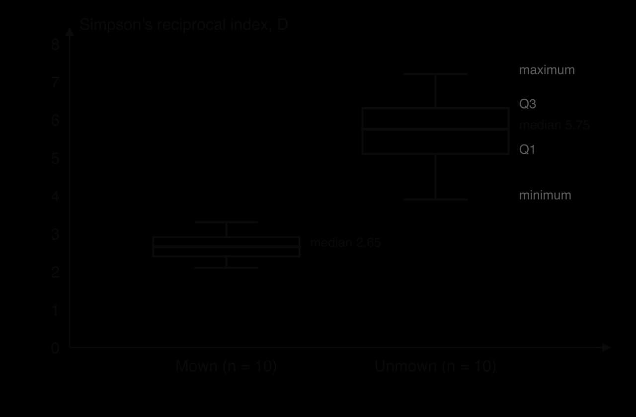
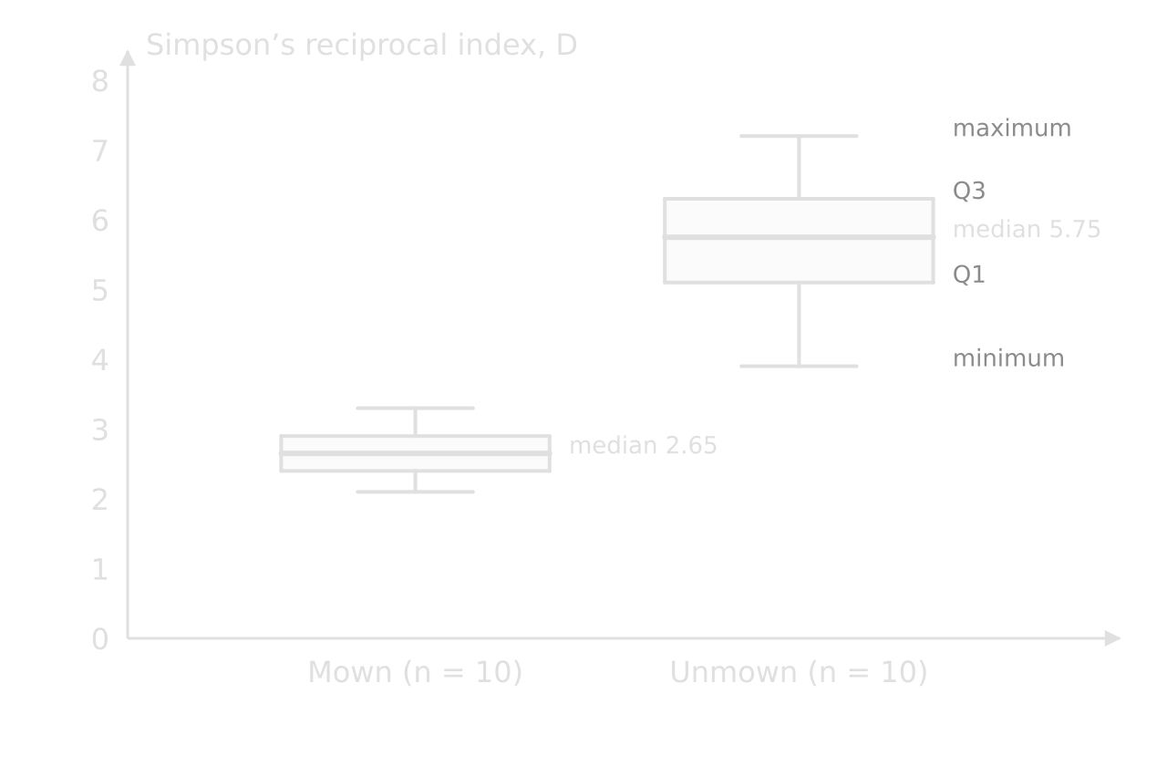
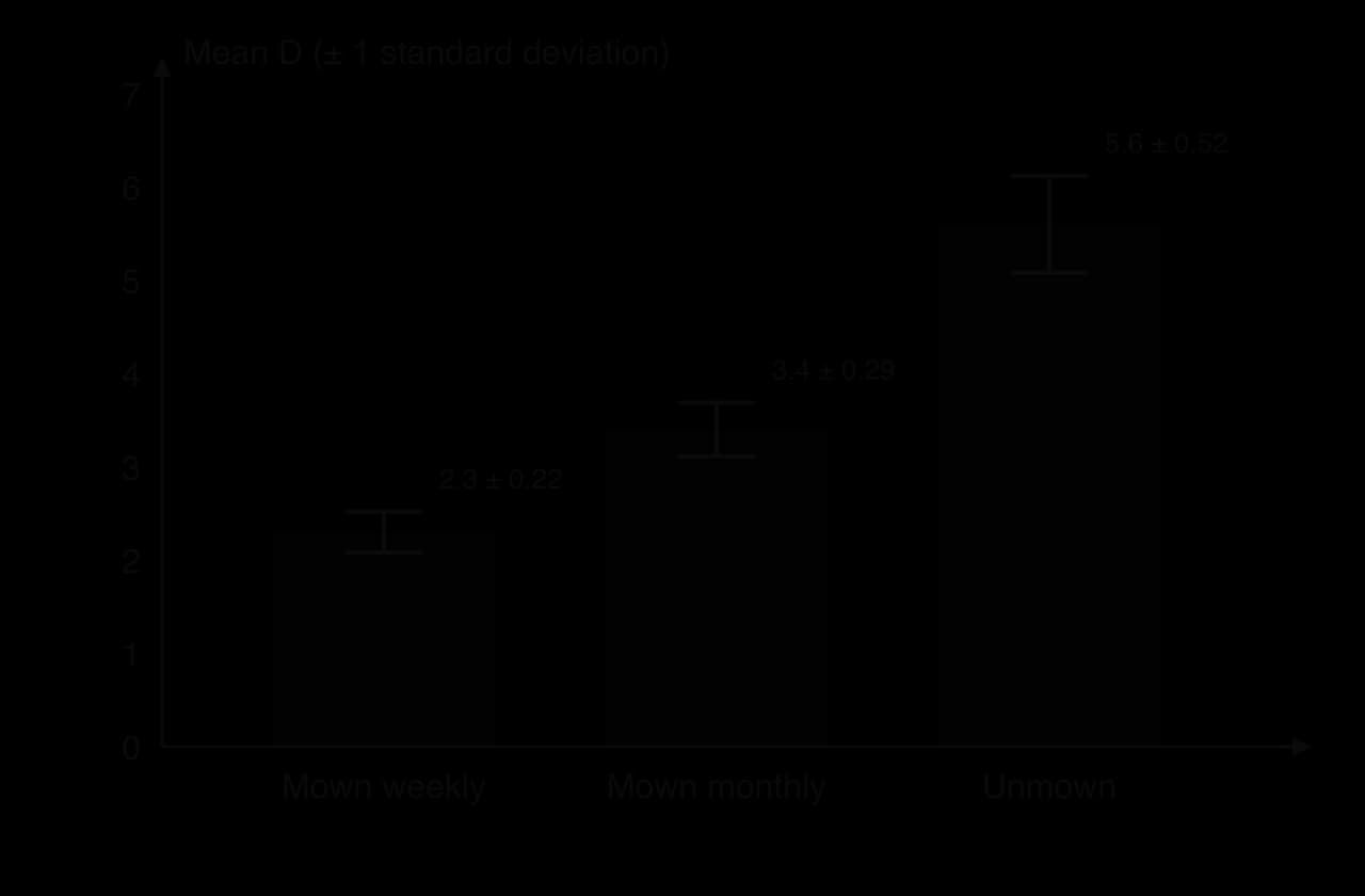
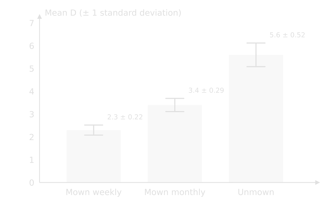
A box and whisker plot is the clearest way to compare two or more groups when the data may be skewed. A column chart of means with error bars does the same job for means: each bar shows the mean, and the error bar shows one standard deviation (or another stated measure) above and below it. Where error bars overlap a lot, a difference between means is unlikely to be significant; where they do not overlap at all, it probably is, although only a statistical test can confirm it.
Choosing the right graph
Purpose | Suitable graph | Example |
|---|---|---|
Compare groups (categories) | Column chart of means with error bars; box and whisker plots | Mean D in mown and unmown grassland |
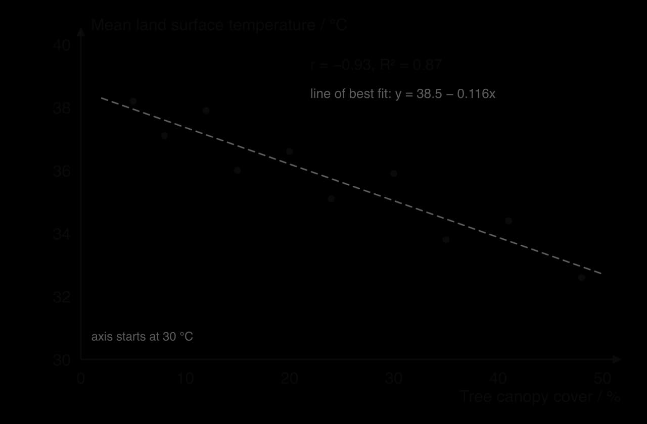
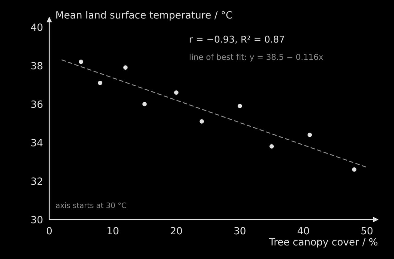
Show a relationship between two continuous variables | Scatter graph with a line of best fit | Tree cover against surface temperature |
Show change along a gradient or over time | Line graph (point to point) or kite diagram for species along a transect | Species richness against distance from a path |
Show parts of a whole | Pie chart or stacked column chart | Percentage of respondents giving each answer |
Show direction | Rose diagram | Wind direction at a monitoring site |
Every graph has a descriptive title (or caption), axes labelled with the quantity and unit, sensible scales, and the independent variable on the x-axis. One clear graph that answers the research question is worth more than six graphs that repeat the same numbers in different forms.
Statistical tests
Descriptive statistics show what the sample looks like. A statistical test asks whether a difference, correlation or association in the sample is large enough, given the variation and the sample size, that it is unlikely to have arisen by chance. If it is, the result is called statistically significant, and the null hypothesis is rejected.
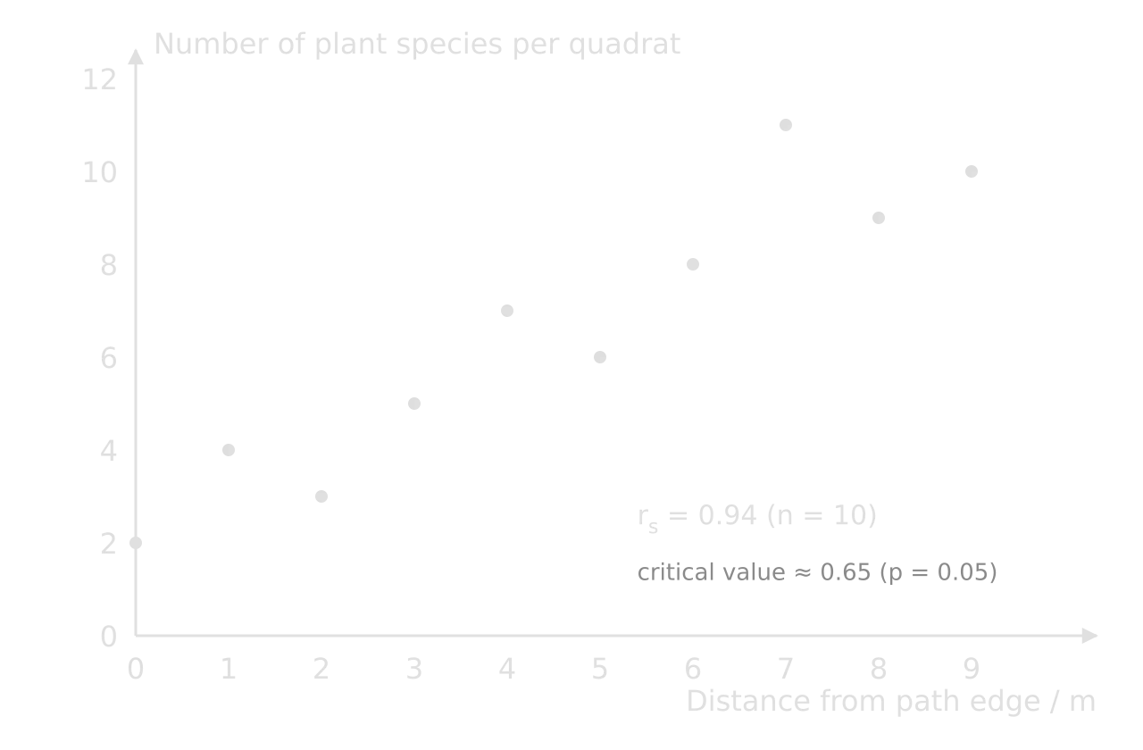
Each test gives a test statistic (t, F, χ², rₛ or r). To decide whether it is significant, the statistic is compared with a critical value from a table, which depends on the chosen significance level (normally p = 0.05) and the degrees of freedom (a number related to the sample size).
If the test statistic is greater than the critical value (for r and rₛ, if its size ignoring the sign is greater), the null hypothesis is rejected. Software gives a p-value instead: the probability of a result at least this extreme if the null hypothesis were true. A p-value below 0.05 means the result is significant at the 5% level.
The t-test: comparing two means
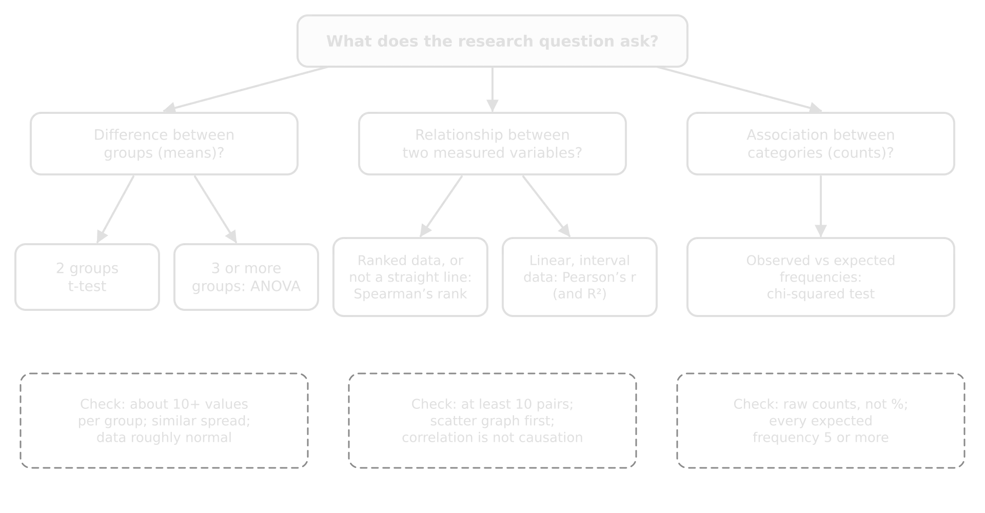
The unpaired t-test compares the means of two independent groups, such as mown and unmown quadrats. It works best with roughly normally distributed data and about ten or more values per group.
ANOVA: comparing three or more means
ANOVA (analysis of variance) compares the means of three or more groups at once. Using several t-tests instead increases the chance of finding a "significant" difference by luck. ANOVA compares the variation between group means with the variation within groups: if the group means are far apart compared with the scatter inside each group, F is large.
The chi-squared test: associations between categories
The chi-squared test compares observed frequencies (counts) with the frequencies expected if there were no association between two categorical variables. It suits survey data such as "support or oppose" against "age group". It must be used on raw counts, never percentages, and every expected frequency should be at least 5.
Spearman's rank: correlation with ranked data
Spearman's rank correlation (rₛ) measures the strength and direction of a correlation between two variables by ranking each and comparing the ranks. It does not need a straight-line relationship or normally distributed data, only that one variable tends to rise (or fall) as the other rises. Values run from +1 (perfect positive) through 0 (none) to −1 (perfect negative).
Pearson's r and R²: linear relationships
The Pearson correlation coefficient (r) measures how closely two continuous variables follow a straight line; like any correlation coefficient, it runs from −1 to +1. It is usually calculated with a spreadsheet (the CORREL function) or a graphing calculator. Its square, the coefficient of determination (R²), gives the proportion of the variation in the dependent variable that is explained by the linear relationship with the independent variable.
Common mistakes in criterion D
Mistake | Fix |
|---|---|
Units missing from headings, or put in every cell | Quantity and unit once in the column heading: "Dissolved oxygen / mg L⁻¹" |
Inconsistent decimal places (2.1, 2.45, 3) | Match the precision of the measurement throughout a column |
Chi-squared on percentages, or with expected values below 5 | Use raw counts; combine categories or collect more responses |
Graphs with default spreadsheet titles ("Series 1") and no axis labels | A descriptive title, labelled axes with units, a legend only when needed |
 YouTube
Checklist for criterion D
- To do:
Raw data tables have titles, headings with units, consistent precision and qualitative notes; a sample is shown, the rest in an appendix.
- To do:
One worked example of each calculation is shown (e.g. one value of D).
- To do:
Processed data include means (or medians) and a measure of spread for each group.
- To do:
Graphs suit the data, with titles, labelled axes, units and stated error bars.
- To do:
A suitable statistical test is chosen and justified, with hypotheses, the statistic, degrees of freedom or n, and the critical value or p-value.
- To do:
The processing answers the research question directly.
Criterion E: analysis and conclusion
Criterion E assesses how well you interpret the data in ways relevant to the research question: the patterns are highlighted, interpreted correctly and used to reach a valid conclusion.
Band | Analysis | Conclusion |
|---|---|---|
1–2 | Identifies patterns or trends relevant to the research question | Does not address the research question, or is not supported by the analysis |
3–4 | Describes relevant patterns or trends, including some measures of bias, reliability, validity and uncertainty | Addresses the research question and is partially supported by the analysis |
5–6 | Explains all relevant patterns and trends, including measures of bias, reliability, validity and uncertainty | Addresses the research question and is supported by the analysis |
Three features move an analysis into the top band. It explains the patterns (gives the ecological, physical or social reasons for them) rather than only describing them. It deals with all the relevant patterns, including the awkward ones (the outlier, the unexpected spread, the group that did not behave as predicted). And it judges the quality of the data, through bias, reliability, validity and uncertainty, before deciding how far the conclusion can be trusted.
Identify, describe, explain
Level | Example from the worked investigation |
|---|---|
Identifies | "Unmown grassland had higher diversity." |
Describes | "Mean D was 5.65 in unmown grassland and 2.65 in mown grassland, more than twice as high, and the difference was significant (t = 8.86, df = 18, p < 0.001). Unmown quadrats were also more variable (SD 1.01 against 0.37)." |
Explains | "Mowing every two weeks removes the leaves and flowering stems of taller species, so only low-growing rosette plants such as daisy and dandelion persist, and they dominate the counts; this keeps both richness and evenness, and therefore D, low. Without mowing, taller species such as yarrow and bird's-foot trefoil can establish, and competition is spread among more species. The higher variability in unmown quadrats suggests that the community is still changing after only one season without mowing, with some patches colonised by new species and others still dominated by clover." |
Explanations come from ESS ideas (succession, disturbance, competition, niches, limiting factors, perspectives) and from the published studies in the background. Returning to those studies in the analysis, and saying whether your results agree with them and why they might differ, is one of the clearest signs of a strong analysis.
Bias, reliability, validity and uncertainty
A supported conclusion includes measures of bias, reliability, validity and uncertainty. These four words are often used loosely; in an investigation each has a precise meaning and a practical way to judge it.
Term | Meaning | How to judge it in the worked example |
|---|---|---|
A systematic distortion of the data or results in one direction | Random coordinates reduce sampling bias; counting only broadleaved plants is a source of bias in D | |
The consistency of the results: whether repeated measurements or a repeat of the investigation would give similar values | Spread within each zone (SD); a second count of two quadrats by a partner agreed to within one plant per species | |
Whether the method measures what it claims to measure and the conclusion follows from the data | Does D of broadleaved plants measure "plant diversity"? Are the zones different only in mowing? | |
The range within which the true value is likely to lie, from measurement limits and from sampling | SD and error bars; the p-value; uncertain identifications (two plants recorded as "species A") |
Two further pairs of ideas help to discuss data quality. Accuracy is how close a measurement is to the true value, while precision is how close repeated measurements are to each other (and the smallest division an instrument can read). Random error causes unpredictable scatter around the true value and is reduced by larger samples and repeats; systematic error shifts every value in the same direction (a miscalibrated pH meter, always counting each rooted clover shoot as a separate plant) and is not reduced by repeating the measurement.
An outlier is a value that lies far from the rest of its group. In the worked example, unmown quadrat 9 (D = 3.9) is the lowest in its zone; the field notes record that it lay in a patch of dense white clover. An outlier should be investigated, not deleted: if there is a clear reason it does not belong to the population (an equipment fault, a quadrat placed on a path), it may be excluded with that reason stated; if it is a real part of the variation, it stays in and is explained.
A common rule of thumb treats values more than 1.5 × IQR beyond the quartiles as outliers; by that rule, 3.9 (above 5.1 − 1.8 = 3.3) is not one.
Correlation and causation
A significant correlation shows that two variables change together, not that one causes the other. Tree cover and surface temperature may both be linked to a third factor (wealthier districts may have both more trees and lower building density). Field comparisons are similar: the unmown zone may differ from the mown zone in ways other than mowing. Causation is better supported when there is a known mechanism, when other variables were controlled or monitored, and when the result agrees with experimental studies. The analysis should say how far these conditions are met.
Writing the conclusion
The conclusion answers the research question directly, in one or two sentences, with the key numbers and the result of the statistical test. It states whether the null hypothesis was rejected, links the result to the ESS theory and the published studies, and is honest about how far the data support it, given the bias, reliability, validity and uncertainty already discussed. A short final link back to the strategy from criterion B ("the results support the council's policy, at least in its first year") is valuable, as long as it does not claim more than the data show.
A weak conclusion on the same data shows how easily a conclusion can claim more than the data allow.
Checklist for criterion E
- To do:
Every relevant pattern and trend is described with numbers from the processed data, including spread and any outliers.
- To do:
Each pattern is explained using ESS theory and compared with the published studies from the background.
- To do:
The result of the statistical test is interpreted in words, with the outcome for the null hypothesis.
- To do:
Bias, reliability, validity and uncertainty are each discussed with evidence from the investigation.
- To do:
Correlation is not presented as causation.
- To do:
The conclusion answers the research question directly, with key numbers, and claims no more than the data support.
Criterion F: evaluation
Criterion F assesses how well you evaluate the investigation itself: the method, the data and the conclusion that rests on them.
Band | Weaknesses and limitations | Improvements | Unresolved questions |
|---|---|---|---|
1–2 | States generic weaknesses or limitations that affect the conclusion | States improvements that address them | States generic questions arising from the investigation |
3–4 | Describes weaknesses or limitations that affect the conclusion | Describes improvements that address them | Outlines questions arising from the investigation |
5–6 | Evaluates specific weaknesses or limitations that affect the conclusion | Evaluates improvements that address them | Describes questions arising, as they affect the conclusion |
Two distinctions matter. A generic weakness could apply to almost any investigation ("human error", "more time", "a bigger sample"); a specific weakness belongs to this method and this data ("grasses were not counted, so D does not include the most abundant plants in either zone"). And there is a difference between methodological weaknesses and limitations.
Methodological weakness | Limitation | |
|---|---|---|
What it is | A problem with how the investigation was carried out: control of variables, or the precision of measurements | A restriction on how far the conclusion can be applied: the range or scope of the data, the boundaries of the system studied, or the assumptions made |
Worked example | Counting individual plants of creeping species (clover, buttercup) is imprecise, because one plant can root at several points | One park, one June, broadleaved plants only: the conclusion cannot be applied to grasses, to other parks or to later years |
Typical improvement | Measure percentage cover for creeping species, or count rooted shoots by a stated rule | Sample several parks, repeat in later summers, include grasses |
The two kinds of problem call for different responses: a weakness is fixed by changing the method, a limitation by widening the scope of the data.
Evaluating, not just listing
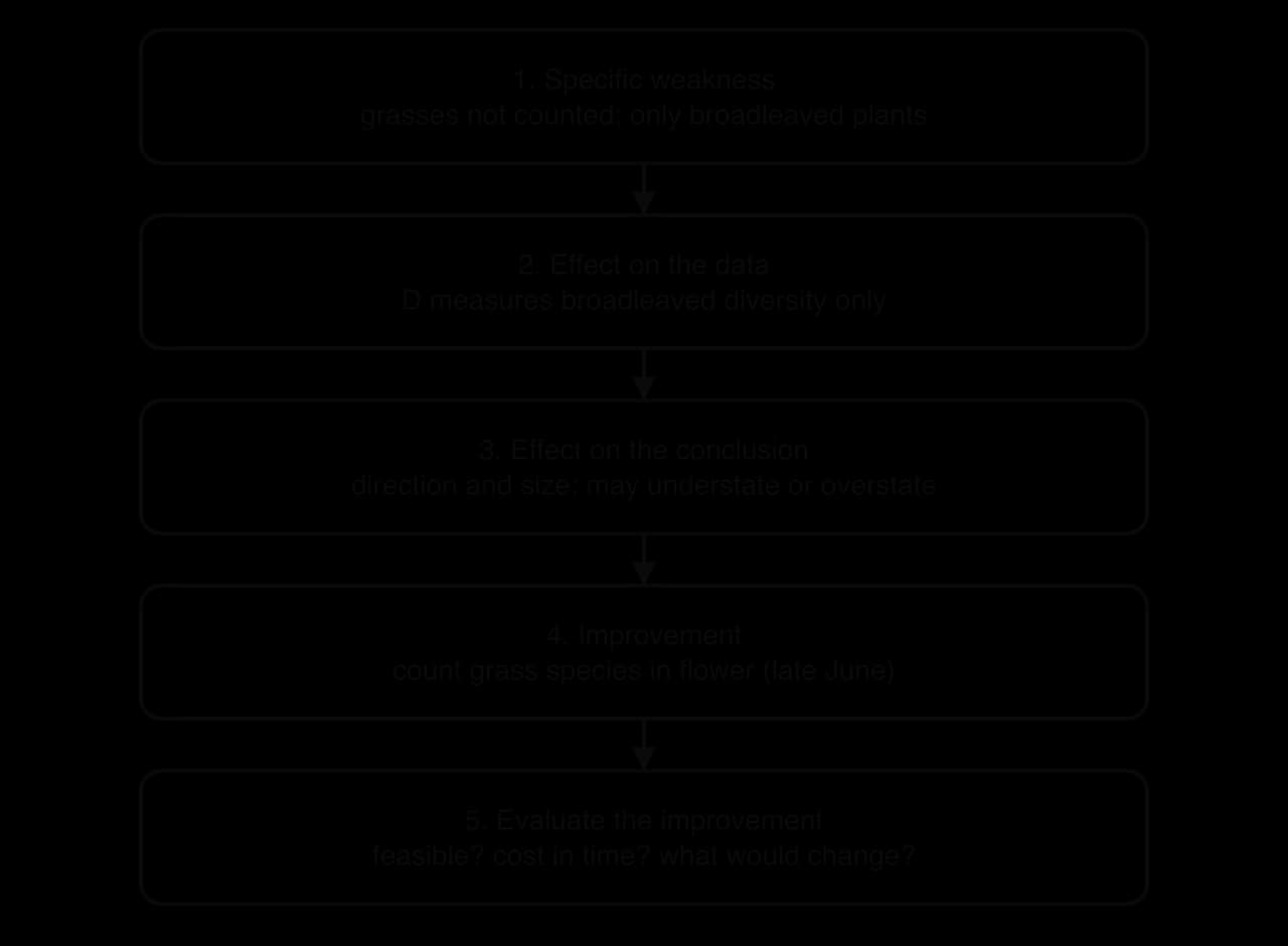
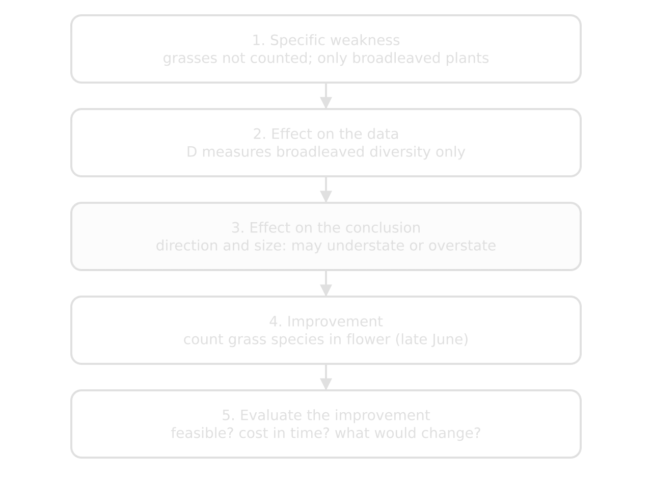
To evaluate a weakness is to judge its importance: how it affected the data, in which direction, how much it matters for the conclusion, and how confident the conclusion can still be. To evaluate an improvement is to judge whether it is realistic, what it would cost in time or equipment, and what difference it would make. Unresolved questions are the questions the investigation could not answer, described in terms of how they affect the conclusion (and, often, the strategy).
Specific weakness or limitation | Effect on data and conclusion | Improvement, evaluated |
|---|---|---|
Grasses not counted (weakness of validity) | D measures broadleaved diversity only. Unmown grassland probably also has more flowering grass species, so the real difference in total plant diversity may be larger; but if tall grasses dominate unmown areas, evenness could be lower. The direction is uncertain, so the conclusion is restricted to broadleaved plants. | Identify grasses from their flowering heads in late June, when most are in flower. Realistic with a grass key and training; adds about 10 minutes per quadrat. |
Counting individuals of creeping species (precision) | One clover plant may be counted as several, inflating n for clover and lowering D in clover-rich quadrats (likely in both zones, so a smaller effect on the difference). | Use percentage cover for creeping species; but D needs counts, so a cover-based index would have to replace D. A clear counting rule (each rooted shoot counts as one) is the more realistic fix. |
Only two zones in one park (limitation of scope) | The zones may differ in ways other than mowing (soil, history, trampling), so the difference cannot be attributed with certainty to mowing alone. | Sample paired mown and unmown areas in three or more parks; the strongest fix, but it triples the fieldwork. |
Unresolved questions arise naturally from these points, and the strongest are tied to the conclusion and the strategy. Does the higher diversity last, increase or fall back after several years of the policy? Does higher plant diversity actually lead to more pollinators, which is the aim of the strategy? Do the gains depend on removing the cut hay, as the council does, or would leaving it make a difference? Each one marks a point at which the conclusion stops.
Checklist for criterion F
- To do:
Three or four specific weaknesses and limitations are chosen, each belonging to this investigation.
- To do:
For each: its effect on the data, the likely direction and size of that effect, and what it means for the conclusion.
- To do:
Each weakness has a realistic improvement, evaluated for feasibility and likely effect.
- To do:
Limitations of scope (one site, one time, one group of organisms or people) are stated as limits on the conclusion.
- To do:
Unresolved questions are described in relation to the conclusion and, where possible, the strategy.
Final checks before submission
- To do:
The title, candidate code(s) and word count are at the top, and the report is within 3,000 words.
- To do:
Each criterion has a clearly headed section.
- To do:
Every number in the analysis and conclusion matches the processed data tables.
- To do:
Every graph and table is referred to in the text.
- To do:
All sources are referenced and the references are complete.
- To do:
The final version takes account of the teacher's comments on the draft.
Carry on with ESS in Augment
With a free account, Augment remembers where you stopped in the notes and which questions you have marked.