Augment Education
    • Question bank
    • Quick fire
    • Worksheets
    • Flashcards
    • Notes
    • Try a quick-fire round
    • All features
    • Business
    • Digital Society
    • Economics
    • Geography
    • Global Politics
    • History
    • Philosophy
    • Psychology
    • Anthropology
    • World Religions
    • Biology
    • Chemistry
    • Physics
    • Computer Science
    • Design Technology
    • ESS
    • SEHS
    • Language and literature
    • Language acquisition
    • Maths AA
    • Maths AI
    • Dance
    • Film
    • Music
    • Theatre
    • Visual Arts
    • Grade calculator
    • Grade boundaries
    • Subject checker
    • Focus timer
    • Exam countdown
    • All free tools
    • IB guide
    • All subjects
  • Blog

Search

Search subjects, the syllabus, glossary terms, the booklets, the IB guide, help and the blog

Log inStart free
augment

Augment Education

IB Diploma revision built around the syllabus.

contact@augment-education.com

Product

  • Features
  • Question bank
  • Quick fire
  • Worksheets
  • Flashcards
  • Notes
  • Subjects
  • What's new

Learn

  • IB guide
  • Booklets, explained
  • Glossary
  • Blog
  • Free tools
  • Grade calculator
  • Subject checker

Company

  • About
  • Help
  • For parents
  • For teachers
  • Comparisons

Subjects

  • English A Lit
  • English A Lang & Lit
  • Chinese A Lit
  • Chinese A Lang & Lit
  • Spanish A Lit
  • Spanish A Lang & Lit
  • English Lit & Perf
  • Spanish Lit & Perf
  • English B
  • Mandarin B
  • Spanish B
  • English ab initio
  • Mandarin ab initio
  • Spanish ab initio
  • Business
  • Digital Society
  • Economics
  • Geography
  • Global Politics
  • History
  • Philosophy
  • Psychology
  • Anthropology
  • World Religions
  • Biology
  • Chemistry
  • Physics
  • Computer Science
  • Design Technology
  • ESS
  • SEHS
  • Maths AA
  • Maths AI
  • Dance
  • Film
  • Music
  • Theatre
  • Visual Arts

Augment Education is developed independently of the International Baccalaureate Organization and is not endorsed by it. “IB” and “International Baccalaureate” are its trademarks.

© 2026 Augment Education. All rights reserved.

  • Privacy
  • Terms
  1. Subjects
  2. Business
  3. Formulae and calculations

Formulae and calculations

Every formula and calculation in the course in one place, grouped by unit, with a short worked example, the units and rounding of each answer and the error students most often make.

  • IB Business Management
  • Exam skills
  • SL and HL

38 min readLast reviewed 15 Oct 2026

Numbers run through every unit of business management: the cost of a workforce, the profit in a set of accounts, the share of a market, the break-even point of a product. Calculations are tested mostly in Paper 2, where most questions are quantitative, and occasionally in Paper 1. HL students meet extra formulas in Paper 2 and use them as evidence in Paper 3 plans.

Every formula and calculation in the course is collected here, unit by unit. Each entry gives the formula in the form examiners expect, a short worked example with invented figures, the unit the answer is written in and the error students most often make. HL-only formulas sit under headings marked "(HL only)". The arithmetic is rarely difficult, and most lost marks come from using the wrong figure, the wrong formula, the wrong unit or no working.

How calculation questions are marked

Calculation questions use the command term "calculate": obtain a numerical answer showing the relevant stages in the working. Because the definition asks for the stages, a typical [2] or [3] calculation gives one mark for the correct method (the right formula with the right figures substituted) and one for the correct answer with its unit. A bare answer that is correct usually earns full marks, but a bare answer that is wrong earns nothing, while a wrong answer with sound working can still earn the method mark.

Many calculations are followed by a second part: "Comment on your answer" [2] or "Explain what your result shows" [2]. In these parts the result is used as evidence. A comment compares the result with something (a previous year, a competitor, a target, a rule of thumb such as a current ratio of 1.5–2) and says what it means for the business in the stimulus material.

  1. Write the formula in words, exactly as on the formula sheet or as learnt.

  2. Substitute the figures from the stimulus, with their units ($000, units, days).

  3. Calculate, keeping full accuracy until the last step.

  4. State the answer with its unit and to the precision asked (2 decimal places for ratios unless told otherwise).

  5. Label what the answer is ("Gross profit margin = 40.00%"), so the examiner can find it at a glance.

Exam tip

Set out every calculation in the five steps, even when the arithmetic feels obvious. It takes about ten seconds longer, protects the method mark if you slip, and lets an examiner award marks for later parts that use your figure.

The own figure rule

Paper 2 questions often build on each other: a contribution per unit is used to find the break-even quantity, which is then used to find the margin of safety. If an early answer is wrong, the later parts are not automatically lost. Under the own figure rule, an examiner marks each later part using the student's own earlier figure, and awards the marks if the method applied to that figure is correct.

Definition

Own figure rule (OFR): the marking principle under which a wrong answer carried forward from an earlier part is not penalised again, so later parts earn marks if the correct method is applied to the student's own figure.

The rule only works if the examiner can see where the figure came from. A later answer of "margin of safety = 900 units" with no working cannot be checked against an earlier mistake, so it earns nothing if it is wrong. Writing "margin of safety = 3,500 − 2,600 = 900 units" earns the mark even though 2,600 was the wrong break-even quantity.

The formula sheet and the formulas to learn

A formula sheet is provided in the exam. It lists the profitability and liquidity ratios, the investment appraisal formulas and, for HL, the efficiency ratios and the capacity utilisation and productivity formulas. HL students are also given a table of discount factors when a question needs one. Every other formula must be learnt, and the table sorts the formulas into the two groups.

Unit

On the formula sheet

Learn it (not on the sheet)

1 Introduction

—

Added value

2 HRM

—

Pay under time rates, piece rates and commission; labour turnover (HL)

3 Finance and accounts

Gross profit margin, profit margin, ROCE (with capital employed); current ratio, acid test ratio; ARR; HL: stock turnover (times and days, with average stock), debtor days, creditor days, gearing ratio, NPV

Total cost, average cost, total revenue, profit; every line of the statement of profit or loss and statement of financial position; cost of sales; working capital; net cash flow and closing balance; payback period; HL: depreciation (straight line, units of production), net book value, variances

4 Marketing

—

Market share, market growth, mark-up price; HL: PED, contribution pricing, moving averages

5 Operations

HL: capacity utilisation rate, productivity rate

Contribution per unit, total contribution, break-even quantity, break-even revenue, profit, margin of safety, target profit output, target price; HL: labour and capital productivity, defect rate, operating leverage, reorder level, cost to buy and cost to make

Toolkit

—

Expected value (decision trees); mean, median, mode, quartiles, standard deviation; relative market share (BCG); HL: total and free float (CPA), overhead allocation (absorption costing), the line y = a + bx (regression)

Tip

Learn the "not on the sheet" column first. The sheet protects you from forgetting a ratio, but nothing protects you from forgetting how to find a break-even quantity or a payback period, and those appear on almost every Paper 2.

Rounding, units and presentation

Rounding and units cost more marks than difficult arithmetic. The conventions examiners use are consistent across the course.

Type of answer

Convention

Example

Ratios given as percentages (margins, ROCE, gearing, ARR, market share, labour turnover, capacity utilisation)

2 decimal places with %

21.18%

Ratios given as a number (current ratio, acid test ratio, stock turnover in times)

2 decimal places; "times" for stock turnover; a ratio may also be written as 2.00 : 1

1.20; 6.55 times

Days (stock turnover in days, debtor days, creditor days)

2 decimal places with "days", unless whole days are asked for

48.67 days

Money

In the unit of the data ($, $000, $m), to the nearest cent for unit prices

$16,500; $32.00 per unit; $240,000

Physical quantities (break-even quantity, target profit output, reorder level)

Whole units; round a break-even or target output up

2,667 units

Payback period

Years and months; months to one decimal place or rounded up

3 years and 3 months

PED

2 decimal places, keeping the minus sign

−1.25

Three habits prevent most rounding errors. Keep full accuracy in the calculator until the final step, and round once. Round a break-even quantity or target profit output up to the next whole unit, because 2,666 units would still leave a small loss when the exact answer is 2,666.67. State the unit in the data: if the stimulus is "in $000", an answer of "360" means $360,000, and should be written "$360,000" or "360 ($000)".

Common mistake

Writing the answer in the wrong unit, such as a gross profit margin of "0.40" instead of 40.00%, or debtor days of "0.13" because the × 365 was left out. Before moving on, ask whether the number is the right kind of number: margins are percentages, liquidity ratios are around 0.5–3, days are usually 10–120.

Negative figures and brackets

In financial statements, cash flow forecasts and budgets, a negative figure or a subtraction is written in brackets: a net cash flow of minus $6,000 is (6) in a forecast "in $000". In a calculation written out in a line, the minus sign is clearer: NPV = $197,155 − $200,000 = −$2,845. A negative net present value, a negative market growth rate or a negative PED is a meaningful answer and keeps its sign.

Using a calculator

A simple four-function calculator is enough for every calculation in the course, and a graphic display calculator is also allowed. Brackets need care, because a calculator follows the standard order of operations and divides before it subtracts.

  • Use brackets for every formula with a sum or difference on top: (current assets − stock) ÷ current liabilities must be entered as (600 − 240) ÷ 300, not 600 − 240 ÷ 300.

  • Store or write down intermediate results in full (average stock, capital employed, contribution per unit) and reuse them, rather than retyping rounded figures.

  • Estimate first. A gross profit of 960 on sales of 2,400 is a little under half, so a margin near 40% is expected; an answer of 4% or 400% shows a slip.

  • Check percentages. Divide, then multiply by 100; the % key on some calculators behaves differently and is best avoided.

Unit 1: Introduction to business management

Added value

Added value is the difference between the price of a product and the cost of the inputs bought in to make it. It measures how much the business itself has contributed through its work, skill and branding.

Added value=price of the output−cost of bought-in inputsAdded value=price of the output−cost of bought-in inputs

Worked example

A furniture maker sells a dining table for $450. The wood, fittings and varnish bought from suppliers cost $170. Calculate the added value per table. [2]

Show the solution

Step 1: write the formula. Added value = price of the output − cost of bought-in inputs.

Step 2: substitute and calculate. $450 − $170 = $280 per table.

Added value is not profit. The $280 still has to pay the maker's wages, rent and other costs; only what is left after those is profit. The common error is to subtract every cost, which gives profit, or to subtract nothing and call the price the added value.

Unit 2: Human resource management

Time rates, piece rates and commission

Pay calculations follow directly from the definitions of each reward. A time rate pays for hours worked; a piece rate pays for units produced; commission pays a percentage of the value of sales, often on top of a basic salary.

Pay (time rate)=hourly rate×hours workedPay (piece rate)=rate per unit×units producedPay (time rate)=hourly rate×hours workedPay (piece rate)=rate per unit×units produced
Pay (salary plus commission)=basic salary+(commission rate×value of sales)Pay (salary plus commission)=basic salary+(commission rate×value of sales)

Worked example

Calculate the weekly or monthly pay of each worker (hypothetical data): (a) a warehouse worker paid $18 an hour for 38 hours; (b) a garment worker paid $0.85 per item who completes 920 items; (c) a sales representative with a basic salary of $1,800 a month and 4% commission on monthly sales of $45,000.

Show the solution

(a) $18 × 38 = $684 for the week.

(b) $0.85 × 920 = $782 for the week.

(c) Commission = 0.04 × $45,000 = $1,800. Pay = $1,800 + $1,800 = $3,600 for the month.

Labour turnover (HL only)

HL only

HL students calculate labour turnover, the percentage of the workforce that leaves in a year, and interpret it.

Labour turnover measures how many employees leave a business in a period, as a percentage of the average size of the workforce.

Labour turnover=number of staff leaving in a yearaverage number of staff×100Labour turnover=average number of staffnumber of staff leaving in a year​×100

Worked example

A hotel group had 240 staff at the start of the year and 260 at the end. During the year 30 staff left. Calculate the labour turnover. [2]

Show the solution

Step 1: average number of staff. (240 + 260) ÷ 2 = 250.

Step 2: labour turnover. (30 ÷ 250) × 100 = 12.00%.

Comment. About one employee in eight left during the year. Whether this is high depends on the industry: hospitality usually has far higher turnover than this, so 12% may suggest good retention.

Common mistake

Dividing by the number of staff at the end of the year, or by the number who joined. The denominator is the average number of staff over the year. Count only leavers in the numerator, not new recruits.

Unit 3: Finance and accounts

Costs, revenue and profit

Every financial calculation starts from three building blocks. Total cost is the sum of fixed and variable costs; total revenue is price multiplied by quantity sold; profit is the difference between them. Average cost is the cost of each unit, and average revenue the revenue per unit, which equals the price when every unit sells at the same price.

Total cost=total fixed costs+total variable costsTotal variable costs=variable cost per unit×quantityTotal cost=total fixed costs+total variable costsTotal variable costs=variable cost per unit×quantity
Average cost=total costoutputTotal revenue=price×quantity soldProfit=total revenue−total costAverage cost=outputtotal cost​Total revenue=price×quantity soldProfit=total revenue−total cost

Worked example

A bakery has fixed costs of $40,000 a month and a variable cost of $6 per cake. It makes and sells 10,000 cakes a month at $12 each. Calculate total cost, average cost, total revenue and profit for the month.

Show the solution

Total variable costs = $6 × 10,000 = $60,000. Total cost = $40,000 + $60,000 = $100,000.

Average cost = $100,000 ÷ 10,000 = $10.00 per cake.

Total revenue = $12 × 10,000 = $120,000.

Profit = $120,000 − $100,000 = $20,000.

Common mistake

Treating fixed costs as a cost per unit. The $40,000 is paid once a month whatever the output, so it is never multiplied by quantity. Average cost falls as output rises precisely because the same fixed costs are spread over more units.

The statement of profit or loss

The statement of profit or loss is a chain of subtractions. Each subtotal is the line above it minus the next cost, in the fixed IB order. Cost of sales is found from stock figures when it is not given directly.

Cost of sales=opening stock+purchases−closing stockCost of sales=opening stock+purchases−closing stock
Gross profit=sales revenue−cost of salesProfit before interest and tax=gross profit−expensesGross profit=sales revenue−cost of salesProfit before interest and tax=gross profit−expenses
Profit before tax=PBIT−interestProfit for period=profit before tax−taxRetained profit=profit for period−dividendsProfit before tax=PBIT−interestProfit for period=profit before tax−taxRetained profit=profit for period−dividends

Worked example

Kestrel Ltd, a sports equipment maker (hypothetical data), reports the following for the year ended 31 December 2025, in $000: sales revenue 2,400; opening stock 200; purchases 1,480; closing stock 240; expenses 600; interest 40; tax 80; dividends 90. Prepare Kestrel's statement of profit or loss. [5]

Show the solution

Step 1: cost of sales. 200 + 1,480 − 240 = 1,440.

Step 2: set out the statement in the IB layout, subtracting line by line.

Kestrel Ltd
Statement of profit or loss for the year ended 31 December 2025

$000

Sales revenue

2,400

Cost of sales

(1,440)

Gross profit

960

Expenses

(600)

Profit before interest and tax

360

Interest

(40)

Profit before tax

320

Tax

(80)

Profit for period

240

Dividends

(90)

Retained profit

150

Step 3: check the arithmetic. 2,400 − 1,440 = 960; 960 − 600 = 360; 360 − 40 = 320; 320 − 80 = 240; 240 − 90 = 150.

Common mistake

Using purchases as cost of sales. Stock bought but not yet sold is still an asset at the year end, so it is not a cost of this year's sales. Adjust for opening and closing stock every time both are given.

The statement of financial position and working capital

The statement of financial position has its own arithmetic. Total assets minus total liabilities gives net assets, which always equals total equity. Working capital is the money available for day-to-day running.

Net assets=total assets−total liabilities=total equityNet assets=total assets−total liabilities=total equity
Working capital=current assets−current liabilitiesWorking capital=current assets−current liabilities

Worked example

At 31 December 2025 Kestrel Ltd has, in $000: property, plant and equipment 1,800; accumulated depreciation 400; cash 40; debtors 320; stock 240; bank overdraft 50; trade creditors 210; other short-term loans 40; long-term borrowings 500; share capital 400; retained earnings 800. Prepare the statement of financial position and calculate working capital.

Show the solution

Kestrel Ltd
Statement of financial position as at 31 December 2025

$000

$000

Non-current assets

Property, plant and equipment

1,800

Accumulated depreciation

(400)

Non-current assets

1,400

Current assets

Cash

40

Debtors

320

Stock

240

Current assets

600

Total assets

2,000

Current liabilities

Bank overdraft

50

Trade creditors

210

Other short-term loans

40

Current liabilities

300

Non-current liabilities

Borrowings—long term

500

Non-current liabilities

500

Total liabilities

800

Net assets

1,200

Equity

Share capital

400

Retained earnings

800

Total equity

1,200

Check: net assets (2,000 − 800 = 1,200) equal total equity (400 + 800 = 1,200), so the statement balances.

Working capital = 600 − 300 = $300,000.

Tip

If net assets and total equity do not match, the error is almost always a misplaced item: an overdraft listed as a non-current liability, or accumulated depreciation added instead of subtracted.

Depreciation (HL only)

HL only

HL students calculate depreciation by the straight line and units of production methods, and the net book value of an asset.

Depreciation spreads the cost of a non-current asset over its useful life. The straight line method charges the same amount every year; the units of production method charges according to how much the asset is used. The net book value is what remains of the cost after the depreciation charged so far.

Annual depreciation (straight line)=cost−residual valueuseful life (years)Annual depreciation (straight line)=useful life (years)cost−residual value​
Depreciation (units of production)=cost−residual valuetotal expected units of output×units produced in the yearDepreciation (units of production)=total expected units of outputcost−residual value​×units produced in the year
Net book value=original cost−accumulated depreciationNet book value=original cost−accumulated depreciation

Worked example

(a) A delivery van costs $48,000, has a residual value of $8,000 and a useful life of 5 years. Calculate the annual depreciation by the straight line method and the net book value at the end of each year. (b) A packing machine costs $64,000, has a residual value of $4,000 and is expected to pack 240,000 units in its life. It packs 70,000 units in year 1 and 90,000 in year 2. Calculate the depreciation for each year by the units of production method.

Show the solution

(a) Annual depreciation = ($48,000 − $8,000) ÷ 5 = $8,000 a year.

End of year

Depreciation ($)

Accumulated depreciation ($)

Net book value ($)

1

8,000

8,000

40,000

2

8,000

16,000

32,000

3

8,000

24,000

24,000

4

8,000

32,000

16,000

5

8,000

40,000

8,000

The net book value at the end of year 5 equals the residual value, which is a quick check.

(b) Rate per unit = ($64,000 − $4,000) ÷ 240,000 = $0.25 per unit. Year 1: 70,000 × $0.25 = $17,500. Year 2: 90,000 × $0.25 = $22,500. Net book value at the end of year 2 = $64,000 − $40,000 = $24,000.

Common mistake

Forgetting to subtract the residual value before dividing. ($48,000 ÷ 5 = $9,600 a year) would depreciate the van to zero, although the business expects to sell it for $8,000.

Profitability ratios

The three profitability ratios are on the formula sheet and should be written exactly as it gives them. Capital employed is the long-term finance in the business: non-current liabilities plus equity.

Gross profit margin=gross profitsales revenue×100Profit margin=profit before interest and taxsales revenue×100Gross profit margin=sales revenuegross profit​×100Profit margin=sales revenueprofit before interest and tax​×100
ROCE=profit before interest and taxcapital employed×100Capital employed=non-current liabilities+equityROCE=capital employedprofit before interest and tax​×100Capital employed=non-current liabilities+equity

Worked example

Using Kestrel Ltd's statements, calculate the gross profit margin, the profit margin and the return on capital employed (ROCE). [4]

Show the solution

Gross profit margin = (960 ÷ 2,400) × 100 = 40.00%.

Profit margin = (360 ÷ 2,400) × 100 = 15.00%.

Capital employed = 500 + 1,200 = 1,700. ROCE = (360 ÷ 1,700) × 100 = 21.18%.

Common mistake

Using profit for period or profit before tax in the profit margin or ROCE. Both formulas use profit before interest and tax, so that businesses with different amounts of borrowing and different tax bills can be compared fairly.

Liquidity ratios

The two liquidity ratios compare what a business can turn into cash quickly with what it must pay soon. The acid test removes stock, the least liquid current asset.

Current ratio=current assetscurrent liabilitiesAcid test (quick) ratio=current assets−stockcurrent liabilitiesCurrent ratio=current liabilitiescurrent assets​Acid test (quick) ratio=current liabilitiescurrent assets−stock​

Worked example

Calculate Kestrel Ltd's current ratio and acid test ratio, and comment on the results. [4]

Show the solution

Current ratio = 600 ÷ 300 = 2.00 (2.00 : 1).

Acid test ratio = (600 − 240) ÷ 300 = 360 ÷ 300 = 1.20 (1.20 : 1).

Comment. Kestrel has $2 of current assets for every $1 of current liabilities, at the top of the commonly quoted range of 1.5–2, and can meet its short-term debts even without selling stock (acid test above 1). Its liquidity is sound; if anything, it may hold more cash and stock than it needs, which could be invested elsewhere.

Liquidity ratios are written as a number to 2 decimal places, not a percentage. The common error is to multiply by 100 out of habit from the profitability ratios.

Efficiency ratios (HL only)

HL only

HL students calculate stock turnover, debtor days, creditor days and the gearing ratio, all given on the formula sheet.

Stock turnover measures how quickly stock is sold, either as a number of times a year or as a number of days. Debtor days and creditor days show how long customers take to pay and how long the business takes to pay its suppliers. The gearing ratio shows how much of the capital employed comes from long-term borrowing.

Average stock=opening stock+closing stock2Average stock=2opening stock+closing stock​
Stock turnover (number of times)=cost of salesaverage stockStock turnover (number of days)=average stockcost of sales×365Stock turnover (number of times)=average stockcost of sales​Stock turnover (number of days)=cost of salesaverage stock​×365
Debtor days=debtorstotal sales revenue×365Creditor days=creditorscost of sales×365Debtor days=total sales revenuedebtors​×365Creditor days=cost of salescreditors​×365
Gearing ratio=non-current liabilitiescapital employed×100Gearing ratio=capital employednon-current liabilities​×100

Worked example

Using Kestrel Ltd's statements (opening stock 200, closing stock 240), calculate stock turnover in times and in days, debtor days, creditor days and the gearing ratio.

Show the solution

Average stock = (200 + 240) ÷ 2 = 220.

Stock turnover = 1,440 ÷ 220 = 6.55 times; in days, (220 ÷ 1,440) × 365 = 55.76 days.

Debtor days = (320 ÷ 2,400) × 365 = 48.67 days.

Creditor days = (210 ÷ 1,440) × 365 = 53.23 days.

Gearing ratio = (500 ÷ 1,700) × 100 = 29.41%.

Comment. Kestrel collects cash from customers about five days faster than it pays its suppliers, which helps its cash flow, and its gearing is in the medium range (25–50%), so further borrowing is possible.

Common mistake

Using sales revenue in the stock turnover or creditor days formulas. Both use cost of sales, because stock and creditors are valued at cost, not at selling price. Only debtor days uses sales revenue.

Cash flow forecasts

A cash flow forecast repeats two calculations for every month. The net cash flow is the difference between total cash inflows and total cash outflows; the closing balance is the opening balance plus the net cash flow, and becomes the next month's opening balance.

Net cash flow=total cash inflows−total cash outflowsClosing balance=opening balance+net cash flowNet cash flow=total cash inflows−total cash outflowsClosing balance=opening balance+net cash flow

Worked example

A café starts March with $15,000 in the bank. It expects cash inflows of $84,000 and cash outflows of $96,000 in March. Calculate the net cash flow and the closing balance for March.

Show the solution

Net cash flow = $84,000 − $96,000 = −$12,000, written (12) in a forecast in $000.

Closing balance = $15,000 + (−$12,000) = $3,000, which is April's opening balance.

Common mistake

Adding the opening balance to the inflows and then calling the result net cash flow. Net cash flow is only this month's inflows minus this month's outflows; the opening balance is added afterwards to give the closing balance.

Payback period

The payback period is the time a project takes to repay its initial cost. It is found from the cumulative cash flow, adding each year's net cash flow to the cost (shown as a negative figure in year 0) until the total turns positive. The months within the payback year assume that the year's cash flow arrives evenly.

Additional months=income neededcontribution per monthcontribution per month=net cash flow in the payback year12Additional months=contribution per monthincome needed​contribution per month=12net cash flow in the payback year​

Worked example

A printing firm buys a machine for $150,000 (hypothetical data). Its forecast net cash flows are $40,000, $50,000, $45,000, $60,000 and $55,000 in years 1 to 5. Calculate the payback period. [3]

Show the solution

Year

Net cash flow ($)

Cumulative cash flow ($)

0

(150,000)

(150,000)

1

40,000

(110,000)

2

50,000

(60,000)

3

45,000

(15,000)

4

60,000

45,000

5

55,000

100,000

Step 1: the cumulative cash flow turns positive in year 4, so payback is 3 full years plus part of year 4.

Step 2: income needed at the start of year 4 = $15,000; contribution per month = $60,000 ÷ 12 = $5,000. Additional months = 15,000 ÷ 5,000 = 3.

Answer: payback period = 3 years and 3 months.

Common mistake

Using the cash flow of the wrong year for the months. The part-year calculation divides by the net cash flow of the year in which payback happens (year 4 here), not the year before it.

Average rate of return

The average rate of return (ARR) is the average annual profit of a project as a percentage of its cost. It is on the formula sheet.

ARR=(total returns−capital cost)÷years of usecapital cost×100ARR=capital cost(total returns−capital cost)÷years of use​×100

Worked example

Calculate the ARR of the printing machine. [2]

Show the solution

Step 1: total returns = 40,000 + 50,000 + 45,000 + 60,000 + 55,000 = $250,000.

Step 2: total profit = $250,000 − $150,000 = $100,000; average annual profit = $100,000 ÷ 5 = $20,000.

Step 3: ARR = (20,000 ÷ 150,000) × 100 = 13.33%.

Common mistake

Forgetting to subtract the capital cost, which gives an ARR of (250,000 ÷ 5) ÷ 150,000 × 100 = 33.33%. Returns that only repay the cost are not profit; the formula divides the profit per year by the cost.

Net present value (HL only)

HL only

HL students calculate net present value using the discount factors provided with the exam.

Net present value (NPV) allows for the time value of money. Each future net cash flow is multiplied by the discount factor for its year and the chosen interest rate to give its present value; the original cost, paid now, is subtracted from the total.

NPV=∑present values of return−original costNPV=∑present values of return−original cost

The discount factors come from a table provided with the paper. The extract shows the rates that appear in it.

Year

4%

6%

8%

10%

20%

1

0.9615

0.9434

0.9259

0.9091

0.8333

2

0.9246

0.8900

0.8573

0.8264

0.6944

3

0.8890

0.8396

0.7938

0.7513

0.5787

4

0.8548

0.7921

0.7350

0.6830

0.4823

5

0.8219

0.7473

0.6806

0.6209

0.4019

Worked example

Using a discount rate of 8%, calculate the NPV of the printing machine. [3]

Show the solution

Year

Net cash flow ($)

Discount factor (8%)

Present value ($)

1

40,000

0.9259

37,036

2

50,000

0.8573

42,865

3

45,000

0.7938

35,721

4

60,000

0.7350

44,100

5

55,000

0.6806

37,433

Total present value

197,155

NPV = $197,155 − $150,000 = $47,155. The NPV is positive, so at 8% the machine earns more than its cost.

Common mistake

Discounting the initial cost, or using the factor for the wrong year. The cost is paid in year 0, so it is subtracted at its full value; the year 1 cash flow uses the year 1 factor, and so on.

Budgets and variances (HL only)

HL only

HL students calculate variances in a budget and label each one favourable [F] or adverse [A].

A variance is the difference between a budgeted figure and the actual figure. Whether it is favourable or adverse depends on the line. For revenue, actual above budget is favourable; for costs, actual above budget is adverse.

Variance=budgeted figure−actual figure, labelled [F] or [A]Variance=budgeted figure−actual figure, labelled [F] or [A]

Worked example

A small studio budgeted for sales revenue of $80,000, materials of $30,000, salaries and wages of $25,000 and rent of $10,000 for the quarter. Actual figures were $86,000, $33,500, $24,200 and $10,000. Calculate the variances. [4]

Show the solution

All figures in $000

Budgeted figures

Actual figures

Variance

Sales revenue

80.0

86.0

6.0 [F]

Total revenues

80.0

86.0

6.0 [F]

Materials

30.0

33.5

3.5 [A]

Salaries and wages

25.0

24.2

0.8 [F]

Rent

10.0

10.0

0.0

Total costs

65.0

67.7

2.7 [A]

Excess of revenues over costs

15.0

18.3

3.3 [F]

Sales were $6,000 above budget, which is favourable; materials cost $3,500 more than planned, which is adverse. The excess of revenues over costs was $3,300 higher than planned.

The common error is to label a variance by its sign alone. A cost that came in $800 below budget is favourable even though actual is the smaller number; write the size of each variance and its label, and check the label against the type of line.

Unit 4: Marketing

Market share and market growth

Market share is a firm's sales as a percentage of total sales in the market. Market growth is the percentage change in the size of the market from one period to the next.

Market share=firm’s salestotal sales in the market×100Market share=total sales in the marketfirm’s sales​×100
Market growth=current market size−previous market sizeprevious market size×100Market growth=previous market sizecurrent market size−previous market size​×100

Worked example

The market for plant-based yoghurt in a country was worth $21.5 million in 2024 and $24.0 million in 2025. One brand sold $3.6 million in 2025. Calculate (a) the brand's market share in 2025 and (b) market growth in 2025. [4]

Show the solution

(a) Market share = (3.6 ÷ 24.0) × 100 = 15.00%.

(b) Market growth = ((24.0 − 21.5) ÷ 21.5) × 100 = (2.5 ÷ 21.5) × 100 = 11.63%.

Common mistake

Dividing by the new market size in a growth calculation. Growth is always measured against the previous period: (24.0 − 21.5) ÷ 24.0 would give 10.42%, which understates it.

Mark-up pricing

Cost-plus pricing adds a percentage mark-up to the cost of each unit. The mark-up can also be found backwards from a price.

Price=unit cost×(1+mark-up %)Mark-up %=price−unit costunit cost×100Price=unit cost×(1+mark-up %)Mark-up %=unit costprice−unit cost​×100

Worked example

A shop buys notebooks at $8.00 each and adds a 35% mark-up. Calculate the selling price. [2]

Show the solution

Price = $8.00 × (1 + 0.35) = $8.00 × 1.35 = $10.80. Check: (10.80 − 8.00) ÷ 8.00 × 100 = 35%.

Mark-up is a percentage of cost, while the gross profit margin is a percentage of sales revenue. A 35% mark-up gives a gross margin of only 2.80 ÷ 10.80 × 100 = 25.93%, and mixing up the two is a frequent error.

Price elasticity of demand (HL only)

HL only

HL students calculate price elasticity of demand and use it to predict the effect of a price change on revenue; contribution pricing also belongs here.

Price elasticity of demand (PED) compares the percentage change in quantity demanded with the percentage change in price. It is normally negative, and its size (ignoring the sign) shows whether demand is elastic (greater than 1) or inelastic (less than 1).

PED=% change in quantity demanded% change in price% change=new−originaloriginal×100PED=% change in price% change in quantity demanded​% change=originalnew−original​×100

Worked example

A bike-repair shop raises the price of a service from $25 to $28. Monthly services fall from 4,000 to 3,400. Calculate the PED and comment on the effect on revenue. [4]

Show the solution

Step 1: % change in quantity = ((3,400 − 4,000) ÷ 4,000) × 100 = −15%.

Step 2: % change in price = ((28 − 25) ÷ 25) × 100 = +12%.

Step 3: PED = −15 ÷ 12 = −1.25.

Comment. Demand is price elastic (1.25 is greater than 1), so the price rise reduces revenue: from $25 × 4,000 = $100,000 to $28 × 3,400 = $95,200.

Contribution pricing sets the price at the variable cost per unit plus a chosen contribution towards fixed costs and profit. A product with a variable cost of $14 per unit and a target contribution of $6 per unit is priced at $14 + $6 = $20.

Common mistake

Putting price on top. PED is quantity over price: % change in quantity demanded ÷ % change in price. Inverting it turns an elastic −1.25 into an inelastic −0.80 and reverses the conclusion about revenue.

Moving averages (HL only)

HL only

HL students forecast sales with moving averages: three-period averages, and four-quarter averages that are then centred.

A moving average smooths out short-term ups and downs to show the trend. Each three-period average is the mean of three consecutive values, placed against the middle one; the window then moves on by one period.

Three-period moving average=sum of three consecutive values3Three-period moving average=3sum of three consecutive values​

Worked example

Monthly sales (units) were 120, 135, 141, 150, 162 and 171. Calculate the three-month moving averages.

Show the solution

(120 + 135 + 141) ÷ 3 = 132; (135 + 141 + 150) ÷ 3 = 142; (141 + 150 + 162) ÷ 3 = 151; (150 + 162 + 171) ÷ 3 = 161. The trend is rising by about 10 units a month.

With quarterly data, four-quarter moving averages fall between two quarters, so each pair is averaged again to give a centred moving average that lines up with a quarter. The seasonal variation for a quarter is the actual value minus the centred trend value.

Unit 5: Operations management

Break-even analysis

Break-even calculations all start from the contribution per unit: the price minus the variable cost per unit, which is what each sale contributes towards fixed costs and then profit.
Contribution per unit=price−variable cost per unitTotal contribution=contribution per unit×quantity soldContribution per unit=price−variable cost per unitTotal contribution=contribution per unit×quantity sold
Profit=total contribution−fixed costsProfit=total contribution−fixed costs
Break-even quantity=fixed costscontribution per unitBreak-even revenue=break-even quantity×priceBreak-even quantity=contribution per unitfixed costs​Break-even revenue=break-even quantity×price
Margin of safety=actual output−break-even quantityMargin of safety=actual output−break-even quantity
Target profit output=fixed costs+target profitcontribution per unitTarget price=fixed costs+target profitoutput+variable cost per unitTarget profit output=contribution per unitfixed costs+target profit​Target price=outputfixed costs+target profit​+variable cost per unit

Worked example

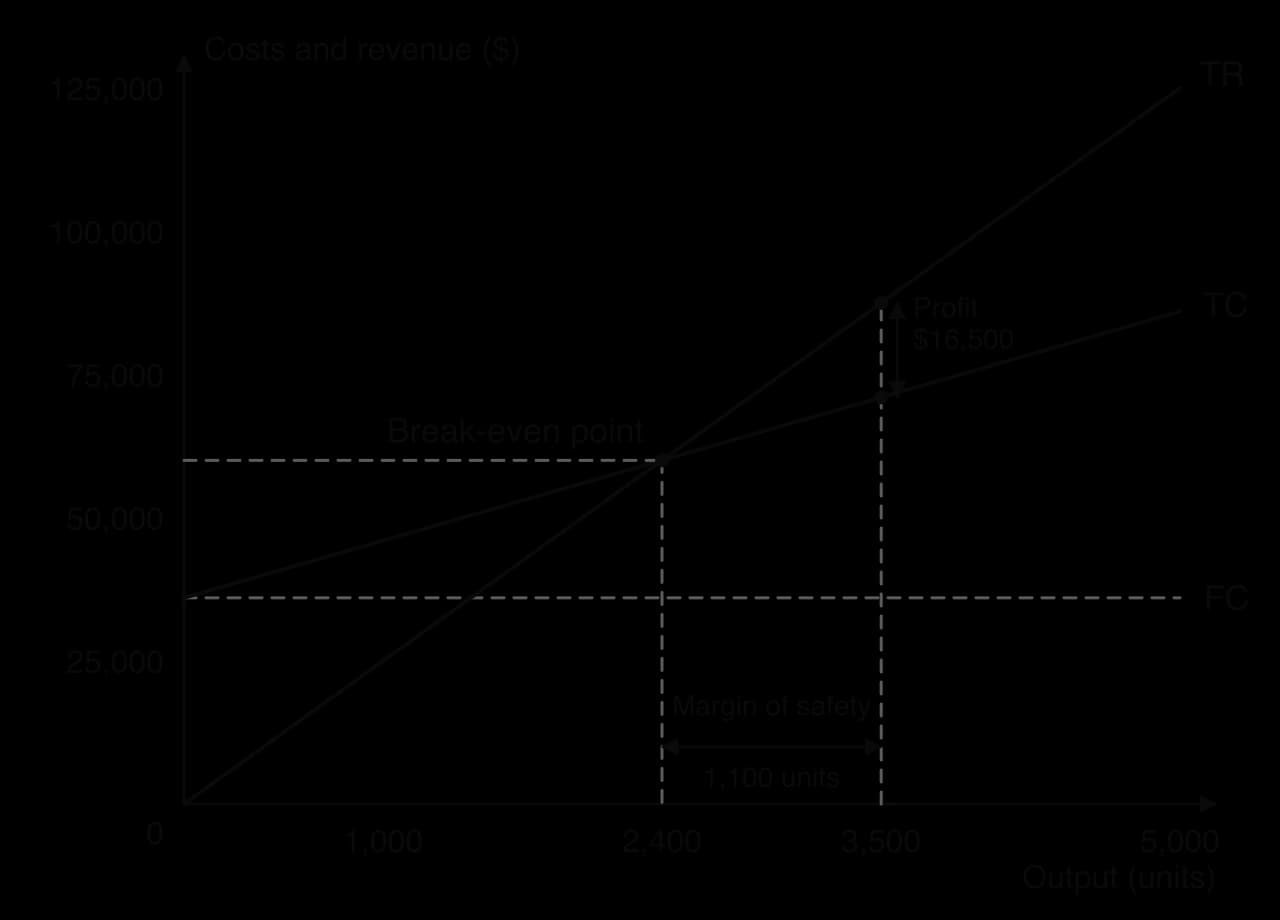
A firm makes water filters. The price is $25, the variable cost is $10 per filter and fixed costs are $36,000 a year. It expects to sell 3,500 filters. Calculate (a) the break-even quantity and break-even revenue; (b) the profit and the margin of safety at 3,500 filters; (c) the output needed for a target profit of $30,000; (d) the target price needed to make $30,000 profit if only 3,000 filters can be sold.

Show the solution

Contribution per unit = $25 − $10 = $15.

(a) Break-even quantity = 36,000 ÷ 15 = 2,400 filters. Break-even revenue = 2,400 × $25 = $60,000.

(b) Profit = (15 × 3,500) − 36,000 = 52,500 − 36,000 = $16,500. Margin of safety = 3,500 − 2,400 = 1,100 filters.

(c) Target profit output = (36,000 + 30,000) ÷ 15 = 4,400 filters.

(d) Target price = (36,000 + 30,000) ÷ 3,000 + 10 = 22 + 10 = $32.00.

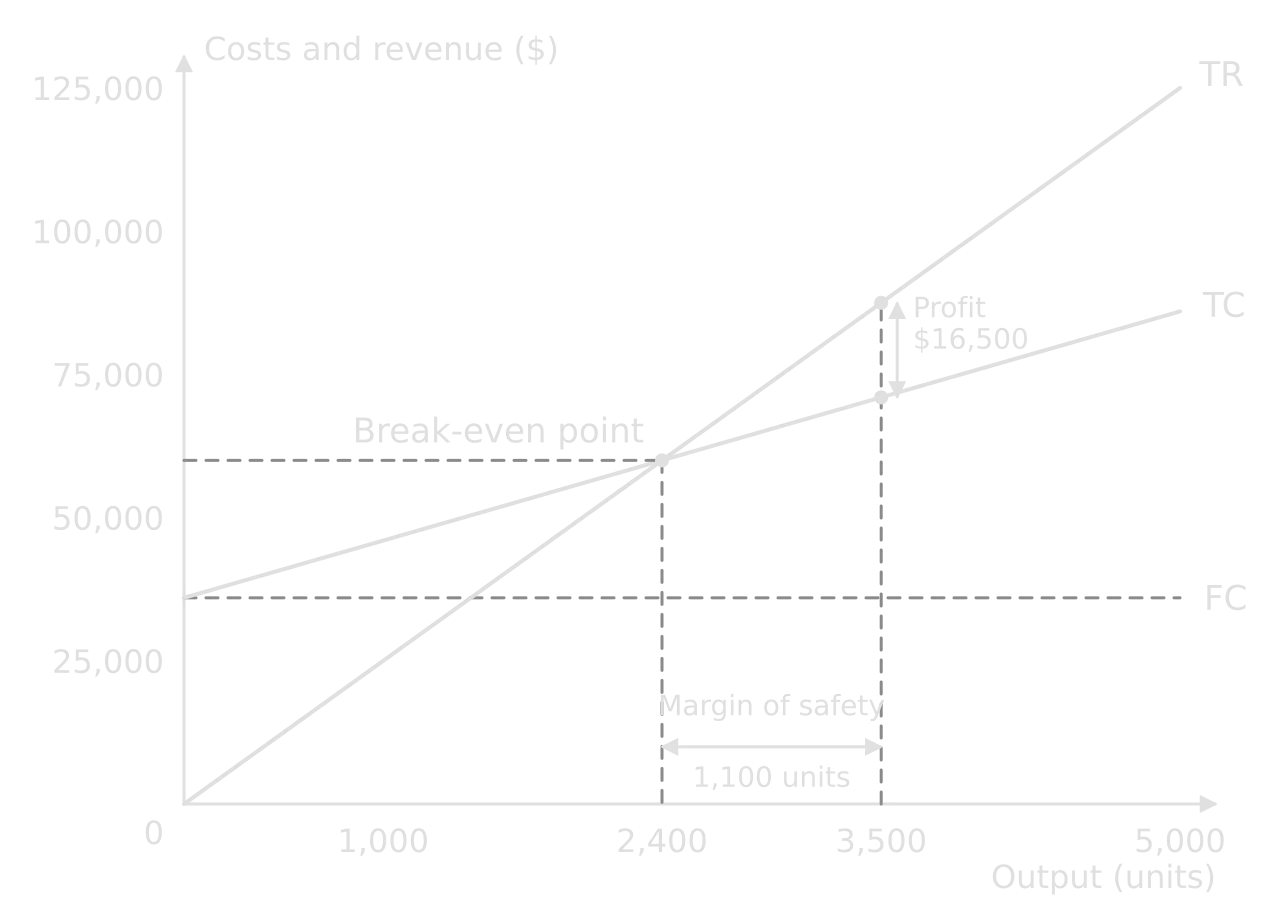
Break-even chart: FC flat at $36,000; TC rises from $36,000 to $86,000 at 5,000 units; TR from 0 to $125,000. Break-even point at 2,400 units and $60,000. At 3,500 units profit is $16,500 and the margin of safety is 1,100 units.Break-even chart: FC flat at $36,000; TC rises from $36,000 to $86,000 at 5,000 units; TR from 0 to $125,000. Break-even point at 2,400 units and $60,000. At 3,500 units profit is $16,500 and the margin of safety is 1,100 units.
Every break-even formula has a place on the chart: TR and TC cross at 2,400 units, the margin of safety is the horizontal gap to actual output, and profit is the vertical gap between TR and TC.

The break-even chart for the water filters shows the same results. Total revenue (TR) and total cost (TC) cross at 2,400 filters and $60,000. At 3,500 filters the vertical distance between TR ($87,500) and TC ($71,000) is the $16,500 profit, and the horizontal distance from the break-even quantity is the margin of safety of 1,100 filters.

Common mistake

Dividing fixed costs by the price instead of the contribution per unit (36,000 ÷ 25 = 1,440). The price does not all go towards fixed costs, because $10 of each sale pays for the filter's own materials and labour.

Capacity utilisation and productivity (HL only)

HL only

HL students calculate capacity utilisation, the productivity rate, labour and capital productivity, the defect rate and operating leverage.

Capacity utilisation compares actual output with the most that could be produced. The productivity rate compares total output with total input, both measured in comparable terms, often their value in money. Labour productivity and capital productivity measure output per unit of one input. The defect rate is the percentage of output that is faulty.

Capacity utilisation rate=actual outputproductive capacity×100Productivity rate=total outputtotal input×100Capacity utilisation rate=productive capacityactual output​×100Productivity rate=total inputtotal output​×100
Labour productivity=total outputlabour inputCapital productivity=total outputcapital inputDefect rate=number of defective unitstotal number of units produced×100Labour productivity=labour inputtotal output​Capital productivity=capital inputtotal output​Defect rate=total number of units producednumber of defective units​×100

Worked example

In one week a factory with a productive capacity of 9,000 units makes 7,200 units, using 30 workers and 160 machine hours; 216 of the units are defective. The output is worth $540,000 and the inputs cost $450,000. Calculate capacity utilisation, the productivity rate, labour productivity, capital productivity and the defect rate.

Show the solution

Capacity utilisation = (7,200 ÷ 9,000) × 100 = 80.00%.

Productivity rate = (540,000 ÷ 450,000) × 100 = 120.00%, so each $1 of inputs produces $1.20 of output.

Labour productivity = 7,200 ÷ 30 = 240 units per worker per week.

Capital productivity = 7,200 ÷ 160 = 45 units per machine hour.

Defect rate = (216 ÷ 7,200) × 100 = 3.00%.

Operating leverage shows how sensitive profit is to a change in sales, and is greater when fixed costs are a large share of total costs. The degree of operating leverage compares the two percentage changes.

Degree of operating leverage=% change in profit before interest and tax% change in sales revenueDegree of operating leverage=% change in sales revenue% change in profit before interest and tax​

If sales revenue rises by 10% and profit before interest and tax rises by 25%, the degree of operating leverage is 25 ÷ 10 = 2.5: each 1% change in sales changes profit by 2.5%, in either direction.

Common mistake

Giving labour or capital productivity as a percentage or without a unit. "240" means nothing; "240 units per worker per week" shows what was measured. Only the productivity rate, capacity utilisation and the defect rate are percentages.

Stock control (HL only)

HL only

HL students calculate the reorder level and read lead time, buffer stock and reorder quantity from a stock control chart.

The reorder level is the stock level at which a new order must be placed so that it arrives just as stock falls to the buffer stock. It depends on how fast stock is used and the lead time of the supplier. The maximum stock level is the buffer stock plus the reorder quantity.
Reorder level=buffer stock+(usage rate×lead time)Maximum stock level=buffer stock+reorder quantityReorder level=buffer stock+(usage rate×lead time)Maximum stock level=buffer stock+reorder quantity

Worked example

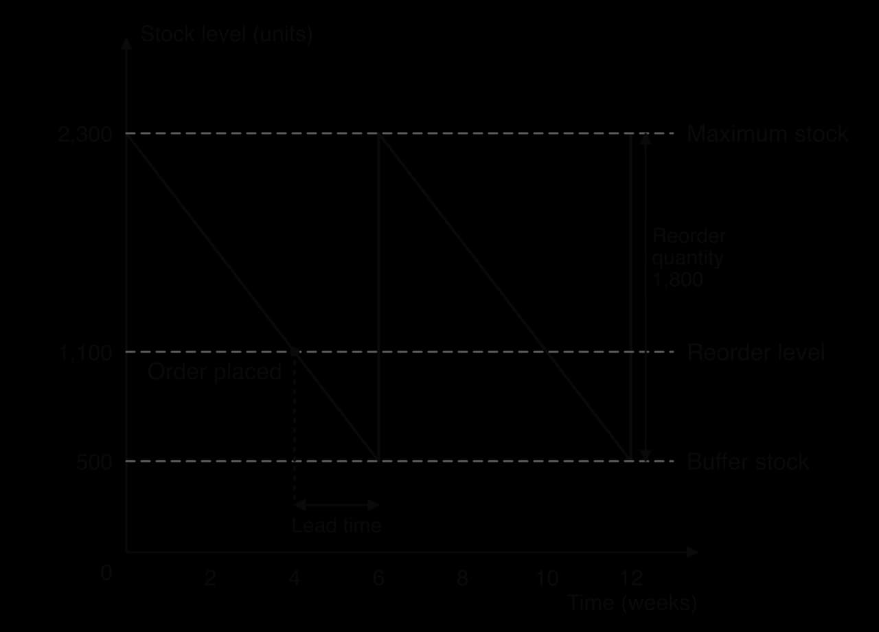
A garden centre keeps a buffer stock of 500 bags of compost, sells 300 bags a week and orders 1,800 bags at a time. Delivery takes 2 weeks. Calculate the reorder level and the maximum stock level. [2]

Show the solution

Reorder level = 500 + (300 × 2) = 1,100 bags.

Maximum stock level = 500 + 1,800 = 2,300 bags.

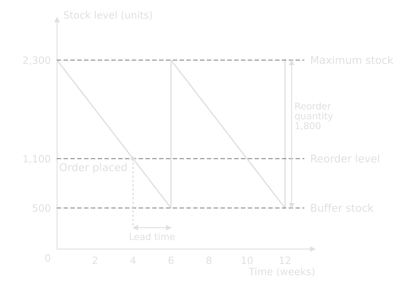
Stock control chart: stock falls 300 units a week from a maximum of 2,300; an order is placed at the reorder level of 1,100 in week 4; after a 2-week lead time stock reaches the buffer of 500 and a reorder quantity of 1,800 restores 2,300.Stock control chart: stock falls 300 units a week from a maximum of 2,300; an order is placed at the reorder level of 1,100 in week 4; after a 2-week lead time stock reaches the buffer of 500 and a reorder quantity of 1,800 restores 2,300.
The order is placed when stock reaches 1,100 bags; during the 2-week lead time 600 bags are sold, so the delivery arrives just as stock reaches the 500-bag buffer.

The stock control chart shows why the formula works. Stock falls from 2,300 to the reorder level of 1,100 in four weeks; the order placed then takes two weeks, during which 600 more bags are sold, and arrives when stock reaches the buffer of 500. The reorder quantity of 1,800 lifts stock back to the maximum.

Cost to buy and cost to make (HL only)

HL only

HL students compare the cost to buy (CTB) a component with the cost to make (CTM) it.

CTB=price per unit×quantityCTM=total fixed costs+(average variable cost×quantity)CTB=price per unit×quantityCTM=total fixed costs+(average variable cost×quantity)

Worked example

A bicycle maker needs 20,000 brackets a year. A supplier charges $4.50 each. Making them would add fixed costs of $30,000 and variable costs of $2.80 per bracket. Calculate the cost to buy and the cost to make. [2]

Show the solution

CTB = $4.50 × 20,000 = $90,000. CTM = $30,000 + ($2.80 × 20,000) = $86,000.

Making the brackets is $4,000 a year cheaper, before qualitative factors such as quality, reliability of supply and the use of the factory's space are considered.

The common error is to compare the supplier's price with the variable cost per unit alone ($4.50 against $2.80), which ignores the extra fixed costs of making the part and makes in-house production look far cheaper than it is.

Business management toolkit

Expected value in decision trees

A decision tree values each option by its expected value: the outcomes at a chance node multiplied by their probabilities and added. The cost of the option is then subtracted to give its net gain. The probabilities at each chance node must add up to 1.

Expected value=∑(probability×outcome)Net gain=expected value−cost of the optionExpected value=∑(probability×outcome)Net gain=expected value−cost of the option

Worked example

Launching a new product costs $150,000. There is a 0.6 probability of high sales, with returns of $500,000, and a 0.4 probability of failure, in which the product loses a further $100,000 before it is withdrawn. The outcomes do not include the launch cost. Calculate the expected value and the net gain of the launch. [3]

Show the solution

Expected value = (0.6 × 500,000) + (0.4 × −100,000) = 300,000 − 40,000 = $260,000.

Net gain = $260,000 − $150,000 = $110,000.

Common mistake

Subtracting the cost inside each branch and then again at the end, so that it is counted twice. Either the outcomes already include the cost (and nothing more is subtracted) or they exclude it (and it is subtracted once at the decision node). Read the stimulus to see which.

Relative market share (BCG matrix)

The horizontal axis of the BCG matrix is relative market share: a product's market share compared with that of the largest competitor. A value above 1 means the product is the market leader.

Relative market share=product’s market sharemarket share of the largest competitorRelative market share=market share of the largest competitorproduct’s market share​

A cereal with 18% of its market, where the largest rival holds 24%, has a relative market share of 18 ÷ 24 = 0.75. The vertical axis is the market growth rate, calculated like market growth.

Descriptive statistics

The mean is the total divided by the number of values; the median is the middle value of ordered data; the mode is the most frequent value. Quartiles split ordered data into quarters, and the interquartile range (IQR) is the spread of the middle half. The standard deviation measures how far values lie from the mean on average.

xˉ=∑xnIQR=Q3−Q1σ=∑(x−xˉ)2nxˉ=n∑x​IQR=Q3​−Q1​σ=n∑(x−xˉ)2​​

Worked example

A food truck's daily sales (in meals) over seven days were 12, 15, 15, 18, 20, 22 and 31. Calculate the mean, median, mode, quartiles, interquartile range and standard deviation.

Show the solution

Mean = 133 ÷ 7 = 19 meals. Median = 4th value = 18. Mode = 15.

Quartiles: lower half 12, 15, 15 gives Q1 = 15; upper half 20, 22, 31 gives Q3 = 22. IQR = 22 − 15 = 7 meals.

Standard deviation: squared differences from the mean are 49, 16, 16, 1, 1, 9 and 144, a total of 236. σ = √(236 ÷ 7) = √33.71 = 5.81 meals.

The mean (19) is above the median (18) because one high day (31) pulls it up; for skewed data like this the median and IQR describe a typical day better.

Float in critical path analysis (HL only)

HL only

HL students calculate the total float and free float of activities in a critical path network.

In critical path analysis, each node shows its earliest start time (EST) and latest finish time (LFT). Total float is how long an activity can be delayed without delaying the whole project; free float is how long it can be delayed without delaying the next activity. Activities on the critical path have zero float.

Total float=LFT−duration−ESTFree float=EST (next activity)−duration−EST (this activity)Total float=LFT−duration−ESTFree float=EST (next activity)−duration−EST (this activity)

Worked example

Activity F lasts 4 days. Its start node has an EST of 6; its end node has an EST of 12 and an LFT of 14. Calculate the total float and the free float of activity F. [2]

Show the solution

Total float = 14 − 4 − 6 = 4 days.

Free float = 12 − 4 − 6 = 2 days.

Common mistake

Using the LFT and EST of the same node. Total float takes the EST from the node where the activity starts and the LFT from the node where it ends.

Absorption costing (HL only)

HL only

HL students allocate overheads in absorption costing and use contribution to judge special orders.

Absorption costing shares indirect costs among departments or products in proportion to a chosen basis, such as floor space, labour hours or machine hours.

Overhead allocated=department’s share of the basistotal of the basis×total overheadsOverhead allocated=total of the basisdepartment’s share of the basis​×total overheads

Rent of $90,000 shared by floor space between departments of 600 m², 300 m² and 100 m² gives $54,000, $27,000 and $9,000. In contribution costing, a special order is accepted on financial grounds if its price is above the variable cost per unit: 500 units at $18 with a variable cost of $14 add a total contribution of 500 × $4 = $2,000.

Simple linear regression (HL only)

HL only

HL students use a line of best fit to make predictions.

A line of best fit through a scatter diagram can be written as y = a + bx, where a is the value of y when x is zero and b is the change in y for each one-unit rise in x. If weekly sales (y) and advertising spending in $000 (x) follow y = 120 + 4.5x, spending of $30,000 predicts sales of 120 + 4.5 × 30 = 255 units. Predictions outside the range of the data (extrapolation) are less reliable.

Checking an answer in ten seconds

Before moving on from any calculation, a short check catches most slips.

Check

What it catches

Is the answer the right kind of number (percentage, ratio, days, units, $)?

Missing × 100 or × 365; ratio given as a percentage

Is it a sensible size? Margins below 100%, current ratios around 0.5–3, days usually 10–120

Wrong figure in the denominator; inverted formula

Do the statement totals add up and does it balance?

Misplaced lines; brackets ignored

Does the break-even quantity times contribution per unit equal fixed costs?

Wrong contribution per unit

Is the cumulative cash flow negative before the payback year and positive at its end?

Months worked from the wrong year

Do probabilities at each chance node add up to 1?

Misread decision tree data

Profit and cash are different numbers. A business can show a profit in its statement of profit or loss and still run out of cash, because credit sales, stock purchases, loan repayments and capital spending affect cash and profit at different times. Never use a profit figure in a cash flow forecast, or a closing cash balance as profit.

Add to your notes: a single formula page of your own, with every formula in the course in two columns ("on the formula sheet" and "learn it"), with the unit of each answer beside the formula and one line on its common error. Rewrite the second column from memory every few weeks until it is word perfect.

Most calculations lead into an explanation or a recommendation that uses the result as evidence, so practise writing one or two sentences after every calculation saying what the result shows for the business and what it is compared with.

Keep your place

In Augment the notes remember where you stopped and which pages you have finished.

Open in Augment

More IB Business notes

  • Paper 1: the pre-released case studyThe page before this.
  • Paper 2: the quantitative paperThe next page.
  • Business assessmentEach Business paper, the internal assessment and grade boundaries.
  • IB BusinessThe Business syllabus, how it is assessed and every notes page.

Carry on with Business in Augment

With a free account, Augment remembers where you stopped in the notes and which questions you have marked.

Start free