Notes on 12.3 Inferential statistics
Learning objectives
Explain why psychologists use inferential statistics to draw conclusions about populations from samples.
Describe the logic of a significance test, including the null and alternative hypotheses, the significance level and the p-value.
Interpret a reported test result, including one-tailed and two-tailed tests, and state a correctly worded conclusion.
Explain type I and type II errors and the trade-off between them.
Explain how sample size and statistical power affect the conclusions a study can draw.
Compare and contrast statistical significance and practical significance, using effect size as an aid.
Explain how multiple comparisons and p-hacking produce false positives, and how they contributed to the replication crisis.
Evaluate null hypothesis significance testing with reference to measurement, bias and causality.
Analyse inferential statistics in an unfamiliar source and state a conclusion linked to a claim.
Introduction
Inferential statistics are the procedures psychologists use to decide whether a difference or relationship found in a sample is likely to exist in the wider population, or could easily have arisen by chance. Almost every quantitative study in psychology ends with a statement such as “the difference was statistically significant (p < 0.05)”, and that statement has to be read correctly for a finding to be understood and reported accurately.
Inferential statistics belong to the concept of measurement, because a p-value is a measure of how surprising the data would be if nothing were going on. They also bear on causality, since a significant difference in a true experiment is the main evidence that an independent variable caused a change, and on bias, since the way researchers analyse and publish results can fill the research literature with false findings.
Why psychologists need inferential statistics
Psychologists almost never study a whole population. A researcher interested in whether sleep loss impairs memory in adolescents cannot test every adolescent, so they test a sample of perhaps 60 and hope to learn something about the millions they did not test. Descriptive statistics, such as the mean and standard deviation, summarise what happened in that sample. They cannot, by themselves, say whether the same pattern would appear in another sample.
The difficulty is that two samples drawn from the same population almost never give exactly the same results. If 30 well-rested and 30 sleep-deprived students each learn a list of words, the two group means will differ a little even if sleep has no effect at all, simply because the individuals in each group differ. This natural variation between samples is called sampling error. Inferential statistics ask whether the difference actually found is larger than sampling error alone would usually produce.
The two kinds of statistics answer different questions, summarised in the table. A study normally reports both: the means and standard deviations first, then the result of an inferential test.
Descriptive statistics | Inferential statistics | |
|---|---|---|
Question answered | What do the data from this sample look like? | Is the pattern in the sample likely to reflect the population? |
Typical output | Mean, median, standard deviation, percentages, a correlation coefficient | A test statistic and a p-value; a decision about the null hypothesis |
Example | Rested group mean = 14.2 words; sleep-deprived mean = 12.8 words | The difference was significant, t(58) = 2.29, p = 0.026 |
Main limitation | Says nothing about chance or the population | Says nothing about how large or important the effect is |
Inferential statistics rest on an assumption that is easy to forget: the sample should be representative of the population the conclusion is about. A significance test can say that a difference between two groups of British university students is unlikely to be due to chance. It cannot say that the same difference would appear among farmers in Kenya or retirees in Japan. That question belongs to generalisability and to the sampling bias of the original study, which no statistical test can repair.
Hypotheses: what a significance test actually tests
Every significance test begins with two competing statements about the population. The null hypothesis (H₀) states that there is no effect: no difference between conditions, or no relationship between variables, in the population. Any difference in the sample is put down to sampling error. The alternative hypothesis (H₁), sometimes called the experimental hypothesis in an experiment, states that there is a real difference or relationship.
The test is built around the null hypothesis rather than the researcher’s own prediction for a logical reason. A null hypothesis is precise (“the difference is zero”), so it is possible to work out what results would be expected if it were true. An alternative hypothesis such as “sleep loss impairs memory” does not say by how much, so it makes no single prediction that can be checked. The test therefore asks how well the data fit the precise null hypothesis, and rejects it when the fit is poor.
Alternative hypotheses come in two forms. A non-directional (two-tailed) hypothesis predicts a difference or relationship without saying which way it goes: “there is a difference in recall between rested and sleep-deprived students”. A directional (one-tailed) hypothesis predicts the direction: “rested students recall more words than sleep-deprived students”. A directional hypothesis is justified only when theory or earlier research gives good reason to expect a particular direction.
The possible outcomes of a test are worded in terms of the null hypothesis. If the data would be very unlikely under H₀, the researcher rejects the null hypothesis and accepts the alternative. If the data are reasonably likely under H₀, the researcher retains (or “fails to reject”) the null hypothesis. Neither outcome proves anything: a significance test deals in probabilities, so every decision carries some risk of being wrong.
Probability, p-values and the significance level
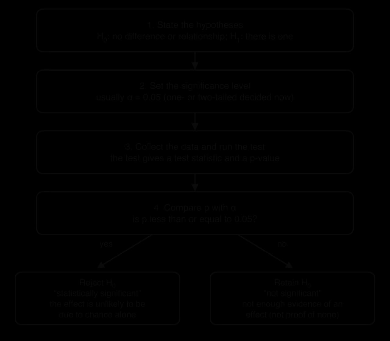
Once the hypotheses are set, the researcher collects data and runs an inferential test. The test compares the size of the effect in the sample with the amount of variation in the data and turns the comparison into a single number, the test statistic. From the test statistic and the sample size it then calculates a probability, the p-value.
The logic runs as follows. The researcher temporarily assumes that the null hypothesis is true and asks how often sampling error alone would produce a difference as large as the one found. If the answer is “very rarely”, either something rare has happened or the null hypothesis is wrong, and researchers choose the second explanation. A p-value of 0.02 means that, if sleep had no effect on memory, a difference at least this large would turn up in only about 2 out of every 100 studies like this one.
Before collecting data, the researcher sets a cut-off called the significance level, written α (alpha). In psychology α is almost always 0.05. If p is less than or equal to α, the result is called statistically significant and the null hypothesis is rejected. If p is greater than α, the result is not significant and the null hypothesis is retained.
Why 0.05, and when a stricter level is used
The 0.05 level is a convention. It became standard in the twentieth century, largely through the influence of the statistician Ronald Fisher, as a reasonable balance between being fooled by chance and missing real effects. A result with p = 0.049 is not meaningfully different from one with p = 0.051, even though one is called significant and the other is not.
Researchers use a stricter level, such as α = 0.01, when a false positive would be costly: when a finding would change medical treatment, contradict a well-established theory, or be used in court. Particle physicists use a far stricter standard still. Benjamin et al. (2018), a group of 72 researchers, proposed that psychology should lower its threshold for new discoveries to 0.005, arguing that 0.05 lets too many false positives into the literature; the proposal was widely debated but not generally adopted.
Sources: Benjamin, D. J. et al. (2018). Redefine statistical significance. _Nature Human Behaviour, 2, 6–10._
Reported p-value | Compared with α = 0.05 | How it is usually worded |
|---|---|---|
p = 0.003 (or p < 0.01) | Smaller | Significant; the null hypothesis is rejected |
p = 0.04 (or p < 0.05) | Smaller | Significant at the 0.05 level; the null hypothesis is rejected |
p = 0.05 | Equal | Significant by the usual convention (p ≤ 0.05), although it is a borderline result |
p = 0.08 | Larger | Not significant; the null hypothesis is retained (sometimes, unwisely, called “a trend”) |
p = 0.62 | Much larger | Not significant; the data are quite consistent with no effect |
This distinction matters so much that in 2016 the American Statistical Association published a formal statement on p-values, listing six principles for using p-values. Two of them address the most common misreadings directly.
P-values do not measure the probability that the studied hypothesis is true, or the probability that the data were produced by random chance alone.
— American Statistical Association, Statement on Statistical Significance and P-Values, principle 2. Wasserstein and Lazar, The American Statistician, 2016
The ASA statement also says that a p-value “does not measure the size of an effect or the importance of a result”, and that scientific conclusions should not be based only on whether a p-value passes a threshold.
 YouTube
Reading and reporting a test result
Published studies report inferential tests in a compact, standard format. A typical sentence reads: “Rested participants recalled more words (M = 14.2, SD = 2.1) than sleep-deprived participants (M = 12.8, SD = 2.6), t(58) = 2.29, p = 0.026.” Each part carries information. The letter (t) names the test statistic, the number in brackets is the degrees of freedom (closely related to the sample size), 2.29 is the value of the test statistic, and p = 0.026 is the probability that leads to the decision.
Reading a result means translating it back into plain language about the variables. The reported sentence says that the difference between the two means is larger than sampling error would usually produce, so the null hypothesis of no difference is rejected at the 0.05 level and the alternative hypothesis is supported: in this sample, sleep deprivation was associated with poorer recall, and the difference is unlikely to be due to chance alone. It does not say how large or important the difference is, which requires the descriptive statistics and an effect size.
Recognising common tests
Many different inferential tests exist, and the choice depends on the design of the study and the type of data. Knowing the names is not essential for interpreting a result, because every test ends in the same way: a test statistic and a p-value. Recognising the name does, however, show what kind of question the researcher asked, which helps in judging whether the conclusion matches the data.
What the study looks for | Design or data | Tests often reported | Test statistic |
|---|---|---|---|
A difference between two conditions | Different participants in each group (independent samples) | Independent t-test; Mann–Whitney U test | t; U |
A difference between two conditions | The same participants in both (repeated measures) | Related (paired) t-test; Wilcoxon signed-rank test | t; T or W |
A difference among three or more conditions | Interval data from several groups | Analysis of variance (ANOVA) | F |
A relationship between two measured variables | Two scores per participant | Pearson’s correlation; Spearman’s rank correlation | r; rho (ρ) |
An association between categories | Counts (frequencies) in categories | Chi-squared test | χ² |
One-tailed and two-tailed tests
The type of alternative hypothesis decides how the 5% risk is spread. A two-tailed test, used with a non-directional hypothesis, splits the 5% between the two ends of the distribution of possible results, so the null hypothesis is rejected if the effect is large in either direction. A one-tailed test, used with a directional hypothesis, puts the whole 5% at one end, so it rejects the null hypothesis only if the effect goes in the predicted direction.
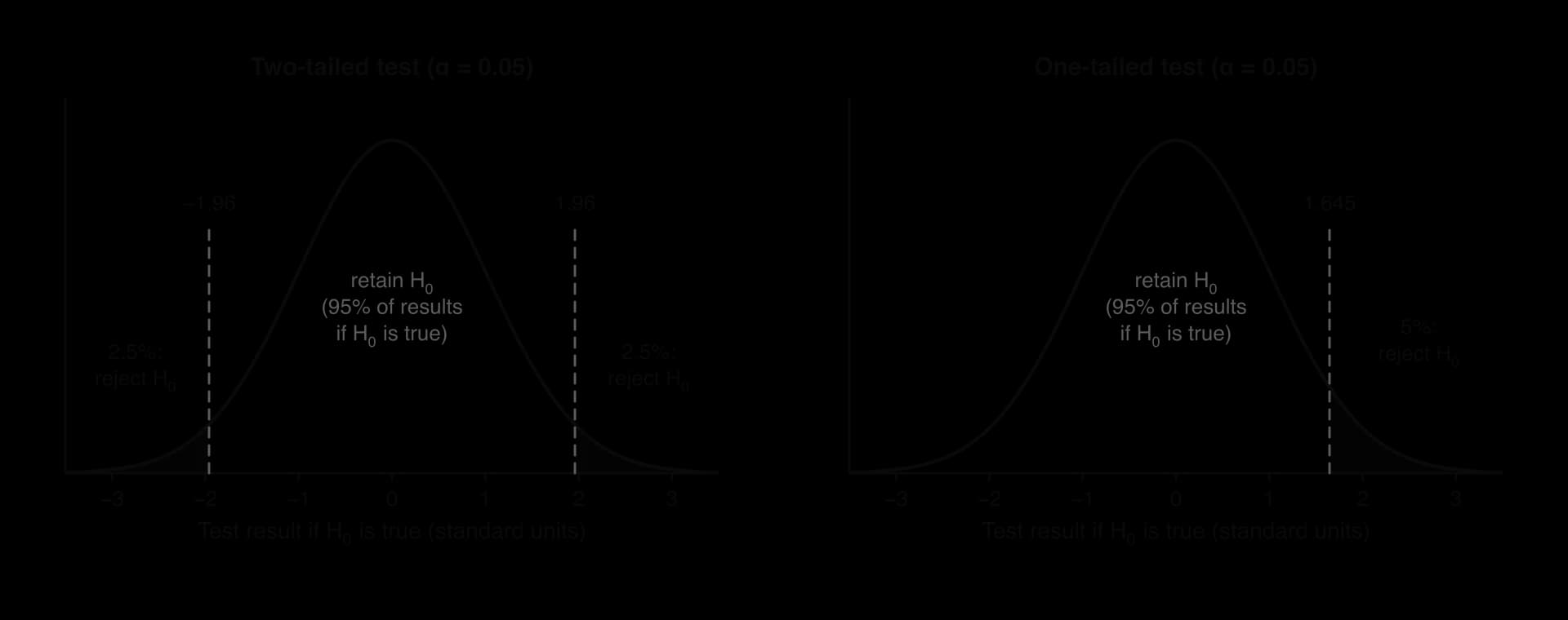
The two curves show why a one-tailed test is more “powerful” in the predicted direction. Because the cut-off is closer to the centre, a result that just misses significance in a two-tailed test can reach it in a one-tailed test. For the same data, the one-tailed p-value is half the two-tailed p-value when the effect is in the predicted direction.
That advantage is also the danger. A one-tailed test is legitimate only if the direction was predicted, for good reasons, before the data were collected, and if an effect in the opposite direction would genuinely be treated as “no effect”. Switching from a two-tailed to a one-tailed test after seeing that p = 0.08 (two-tailed) would become p = 0.04 (one-tailed) is a form of flexible analysis (p-hacking), and it doubles the true risk of a false positive.
Type I and type II errors
Because a significance test deals in probabilities, the decision it leads to can be wrong in two ways. Researchers can conclude that there is an effect when in reality there is none, or conclude that there is no effect when in reality there is one. These are called type I and type II errors.
A type I error (a false positive) happens when the null hypothesis is rejected although it is true. The researcher reports a significant effect that does not exist in the population. Its probability is the significance level: at α = 0.05, about 1 in 20 tests of a true null hypothesis will be significant by chance.
A type II error (a false negative) happens when the null hypothesis is retained although it is false. A real effect exists but the study fails to detect it. Its probability is written β (beta), and it is high when samples are small or effects are small.
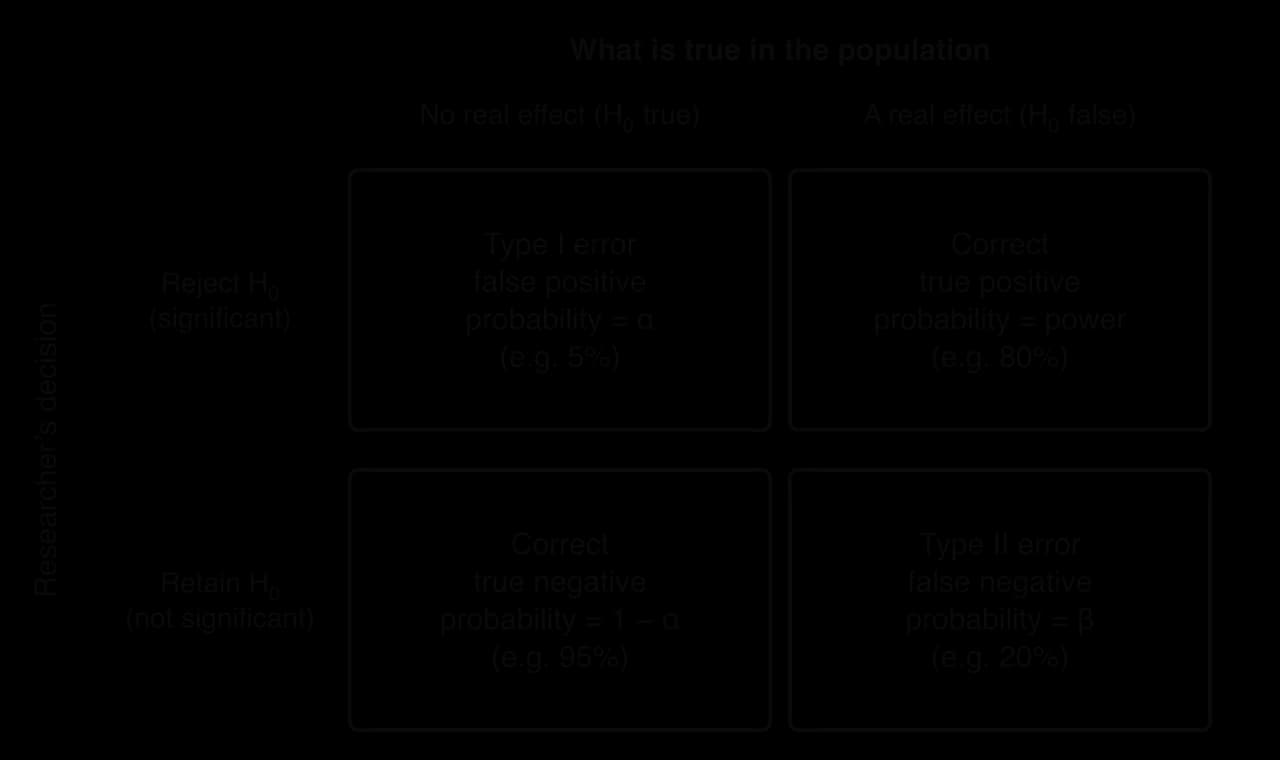
The table shows that each error belongs to one of the two possible states of the world. If there is really no effect (left column), the only possible error is a type I error; if there really is an effect (right column), the only possible error is a type II error. Researchers never know which column they are in, which is why every conclusion from a single study is provisional.
The trade-off between the two errors
The two errors pull against each other. Lowering the significance level from 0.05 to 0.01 makes a type I error less likely, because the result must be more extreme before it counts as significant. But the same change makes a type II error more likely, because some real effects will now fall short of the stricter threshold. Raising α to 0.10 has the opposite effect. With a fixed sample, a researcher can reduce one error only by accepting more of the other.
Change | Risk of type I error | Risk of type II error | When it might be chosen |
|---|---|---|---|
Stricter significance level (α = 0.01) | Falls | Rises | When a false positive would be costly: a new drug, a challenge to an established theory, many tests at once |
More lenient level (α = 0.10) | Rises | Falls | Exploratory pilot research, where missing a possible effect matters more; findings must then be confirmed |
Larger sample size | Unchanged (set by α) | Falls | Whenever it is affordable and ethical: the only way to reduce both errors’ consequences at once |
Which error is worse depends on the consequences. Suppose researchers test whether a cheap online programme reduces adolescent anxiety. A type I error would lead schools to spend time and money on a programme that does not work, and might delay effective help. A type II error would lead a useful programme to be abandoned. In screening for a serious condition, missing a real case (a false negative) is usually treated as the more serious error, so screening tests are deliberately set to produce more false positives, which are then checked.
Sample size and statistical power
A study that cannot detect the effect it is looking for is wasted effort, and possibly unethical, because participants gave their time for nothing. The chance that a study will detect a real effect is called its statistical power. Power is the opposite of a type II error: if β is 20%, power is 80%.
Three things mainly decide power. The first is the size of the real effect: large differences are easy to detect, small ones are hard. The second is the sample size: more participants reduce sampling error, so a real difference stands out more clearly from chance variation. The third is the significance level: a stricter α lowers power. Less variable measures and repeated measures designs, in which each participant acts as their own control, also increase power by reducing the noise in the data.

The curves explain a pattern that runs through psychological research. A study with 20 participants per group has about a 70% chance of detecting a large effect, but only about a 35% chance of detecting a medium one and under 10% for a small one. Most effects in psychology are small to medium, so a field built on small samples will miss many real effects and produce a large number of type II errors.
Researchers can estimate in advance how many participants they need, a step called a power analysis. They decide the smallest effect worth detecting, often from earlier research, choose α and the target power, and calculate the sample size. Funding bodies and journals increasingly ask for this calculation, because it shows that a study was designed to answer its question.
Why underpowered studies also produce false positives
Low power does not only cause missed effects. When an underpowered study does reach significance, the effect it reports is likely to be exaggerated. With a small sample, only an unusually large difference in the data can cross the significance threshold, so the significant studies are those that happened to overestimate the real effect by chance. Among significant results, a higher proportion are also false positives, because real effects are detected so rarely that the 5% of chance findings make up a larger share.
Button et al. (2013) examined 49 meta-analyses in neuroscience and estimated that the median statistical power of the individual studies was only about 21%. A typical study therefore had roughly a one-in-five chance of detecting the effect it was looking for. The authors argued that low power leads to overestimated effects and poor reproducibility, and that it is an ethical problem as well as a statistical one, because unreliable research wastes participants’ time and research funding.
Sources: Button, K. S. et al. (2013). Power failure: why small sample size undermines the reliability of neuroscience. _Nature Reviews Neuroscience, 14, 365–376._
Statistical significance versus practical significance
“Significant” in statistics means “unlikely to be due to chance”, not “large” or “important”. Because the p-value depends on the sample size as well as on the size of the effect, a very large study can make a tiny, trivial difference significant, and a small study can fail to make a large, important difference significant. Interpreting a result therefore needs a second question: how big is the effect, and does it matter in real life?
The size of an effect is measured by an effect size, a number that expresses how large a difference or relationship is in a way that does not depend on the sample size. For a difference between two groups the most common effect size is Cohen’s d, the difference between the means divided by their pooled standard deviation. For a relationship the correlation coefficient r is itself an effect size.
Jacob Cohen suggested rough conventions for d: about 0.2 is small, 0.5 is medium and 0.8 is large. A d of 0.5 means that the two group means are half a standard deviation apart, so the two distributions still overlap a great deal. These labels are only a starting point. In education, health and policy, where outcomes are hard to change, effects that Cohen would call small can be valuable if they apply to many people at low cost.
A national study of a short online growth-mindset lesson shows the difference between the two kinds of significance. Yeager et al. (2019) gave the lesson or a control lesson to a nationally representative sample of more than 12,000 ninth-grade students in 65 US high schools. Among lower-achieving students (n = 6,320), the lesson raised average grades in core subjects by 0.10 grade points (on a 4-point scale), p = 0.001, a standardised effect of 0.11. The result is clearly statistically significant, but the effect is small: whether it is practically significant depends on the low cost of a lesson lasting under an hour and on how many students it could reach.
Sources: Yeager, D. S. et al. (2019). A national experiment reveals where a growth mindset improves achievement. _Nature, 573, 364–369._
Two hypothetical studies of the same mindfulness app for reducing stress make the same point.
Study A | Study B | |
|---|---|---|
Participants | 40 (20 per group) | 4,000 (2,000 per group) |
Reduction in stress score (out of 40) | 6.0 points | 0.5 points |
Effect size (d) | 0.70 | 0.06 |
p-value | 0.03 | 0.04 |
Confidence intervals
Many journals now ask researchers to report a confidence interval alongside the p-value. A 95% confidence interval is a range of values, calculated from the sample, that would contain the true population value in 95% of studies run in the same way. In Yeager et al. (2019) the effect on grades was 0.10 with a 95% confidence interval of 0.04 to 0.16. The interval shows the likely size of the effect (small, but above zero) as well as its significance: an interval for a difference that does not include zero corresponds to a significant result at the 0.05 level.
The multiple comparisons problem
A significance level of 0.05 controls the risk of a false positive for one test. Most studies run many tests: several dependent variables, several groups, several time points, or, in brain imaging, a separate test for each of many thousands of tiny areas of the brain. Each test carries its own 5% risk, so the chance that at least one of them is a false positive grows quickly with the number of tests. This is the multiple comparisons problem.
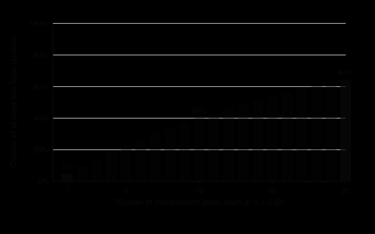
The chart shows that a researcher who tests 20 unrelated questions on random data has nearly a two-in-three chance of finding something “significant” to report. If only that result is published, readers have no way to know it was one of twenty.
The most memorable demonstration came from brain imaging. Bennett, Baird, Miller and Wolford (2010) placed a dead Atlantic salmon in an fMRI scanner and “asked” it to judge the emotions of people shown in a series of photographs. Using a standard uncorrected threshold of p < 0.001, they found a cluster of “active” voxels in the salmon’s brain cavity. When they applied standard corrections for multiple comparisons, no voxels were active, even at relaxed thresholds, showing that the original “activity” was produced by running thousands of separate tests, one per voxel, without correction.
Sources: Bennett, C. M., Baird, A. A., Miller, M. B. & Wolford, G. L. (2010). Neural correlates of interspecies perspective taking in the post-mortem Atlantic salmon: an argument for proper multiple comparisons correction. _Journal of Serendipitous and Unexpected Results, 1(1), 1–5._
Researchers deal with the problem by correcting the significance level. The simplest method, the Bonferroni correction, divides α by the number of tests: with 10 tests, each one must reach p < 0.005 to count as significant, which keeps the overall risk of any false positive near 5%. The cost is lower power, so a corrected study needs a larger sample. Alternatives such as the false discovery rate correction are less strict and are widely used in brain imaging. Another solution is to state in advance one primary hypothesis, so that only one test decides the main conclusion.
p-hacking and the replication crisis
Between about 2011 and 2015 psychologists discovered that many well-known findings could not be reproduced when other researchers repeated the studies. This period, and the reforms that followed it, is known as the replication crisis. Its causes lie largely in how significance testing was used: in the incentives to publish significant results and in the flexibility researchers had in analysing their data.
How flexible analysis creates false positives
p-hacking is the practice of analysing data in many different ways and reporting only the analyses that reach p < 0.05. It is often not deliberate fraud. Researchers face many reasonable-seeming choices, and if each choice is made after seeing which option gives a significant result, the true risk of a false positive rises far above 5%.
Optional stopping: checking the p-value as data come in and stopping as soon as it falls below 0.05.
Selective outcomes: measuring several dependent variables and reporting only the one that worked.
Flexible exclusions: deciding after the analysis which participants count as outliers.
Adding or removing control variables, or splitting the sample into subgroups (by gender, by age) until one shows an effect.
HARKing (hypothesising after the results are known): presenting an unexpected finding as if it had been predicted all along.
Simmons, Nelson and Simonsohn (2011) showed how powerful these choices are. In computer simulations of data with no real effect, combining a few common flexible choices raised the false-positive rate from the nominal 5% to over 60%. In a real experiment they then used the same freedoms to “show” something impossible: that undergraduates who listened to the Beatles song When I’m Sixty-Four were afterwards younger, by their actual age, than those who listened to a control song. The point was not the song but the method: undisclosed flexibility can make almost anything significant.
Sources: Simmons, J. P., Nelson, L. D. & Simonsohn, U. (2011). False-positive psychology: undisclosed flexibility in data collection and analysis allows presenting anything as significant. _Psychological Science, 22(11), 1359–1366._
In the same year, Bem (2011) published nine experiments with more than 1,000 participants in a leading social psychology journal, eight of which gave significant evidence that people could be influenced by events that had not yet happened (precognition). The studies used standard methods and passed peer review. Ritchie, Wiseman and French (2012) then ran three pre-registered replications of one of the experiments with 150 participants in total and found no effect. For many psychologists, the episode showed that the usual standards of evidence could produce significant support for a claim that was almost certainly false.
Sources: Bem, D. J. (2011). _Journal of Personality and Social Psychology, 100(3), 407–425. Ritchie, S. J., Wiseman, R. & French, C. C. (2012). PLoS ONE, 7(3), e33423._
Publication bias and the file drawer
p-hacking interacts with publication bias, the tendency of journals to publish significant results and of researchers to leave non-significant ones unpublished “in the file drawer”. If 20 laboratories test the same false idea and one obtains p < 0.05 by chance, the one significant study may be published while the 19 null results never appear. Readers of the literature then see only the false positive. Several famous effects, including the claim that holding expansive “power poses” for a couple of minutes changes hormone levels, fell apart in this way once larger studies were run.
 YouTube
Reforms after the replication crisis
The response to the crisis, often called the open science movement, aims to remove the flexibility that p-hacking depends on and to make null results visible. The central reform is pre-registration: before collecting data, researchers publish a time-stamped plan stating their hypotheses, sample size, measures and analyses. Any analysis not in the plan must then be reported as exploratory.
A stronger version, the Registered Report, is a journal format in which reviewers judge the introduction and method before the results exist, and the journal agrees to publish the paper whatever the results show. Scheel, Schijen and Lakens (2021) compared 71 Registered Reports with a random sample of 152 standard psychology papers. In the standard papers, 96% of first hypotheses were supported; in the Registered Reports, only 44% were.

The gap in the chart does not prove that half of all standard findings are false, since Registered Reports may tackle riskier questions. It does show that a literature in which almost every hypothesis is confirmed is not a neutral record of what researchers found. Other reforms include sharing data and materials openly, running power analyses, reporting effect sizes and confidence intervals, and large multi-site replications such as the Many Labs projects, which test the same effects in samples from many countries at once.
Sources: Scheel, A. M., Schijen, M. R. M. V. & Lakens, D. (2021). An excess of positive results: comparing the standard psychology literature with Registered Reports. _Advances in Methods and Practices in Psychological Science, 4(2)._
Key study: Open Science Collaboration (2015), estimating the reproducibility of psychology
Aim
The Reproducibility Project: Psychology aimed to estimate how often findings published in leading psychology journals could be reproduced when the studies were repeated as closely as possible with new participants. It was the first large, systematic attempt to measure the replicability of a whole field rather than of single famous effects.
Method
A collaboration of about 270 researchers, coordinated by Brian Nosek and the Center for Open Science, selected studies published in 2008 in three major journals: Psychological Science, the Journal of Personality and Social Psychology and the Journal of Experimental Psychology: Learning, Memory, and Cognition. The Journal of Personality and Social Psychology publishes social psychology, the Journal of Experimental Psychology: Learning, Memory, and Cognition cognitive psychology, and Psychological Science both. One key finding from each of 100 experimental and correlational studies was chosen for replication.
Each replication team contacted the original authors for their materials and asked them to review the planned procedure in advance, so that the replication would be as faithful as possible. Sample sizes were chosen to give high statistical power (at least 80%, and often above 90%) to detect the effect size the original study had reported. The plans were registered before data collection, and all data and materials were made public.
Because there is no single definition of a successful replication, the project measured it in five ways: whether the replication was statistically significant in the same direction; the effect sizes of the original and the replication, both converted to the correlation coefficient r; whether the original effect size fell inside the replication’s 95% confidence interval; whether the replication team judged subjectively that the effect had replicated; and a meta-analysis combining the original and replication data.
Results
Of the original studies, 97% had reported a statistically significant result (p < 0.05). Only 36% of the replications were significant. The mean effect size fell from r = 0.403 (SD = 0.188) in the originals to r = 0.197 (SD = 0.257) in the replications, so the replication effects were on average about half the size of the original ones.
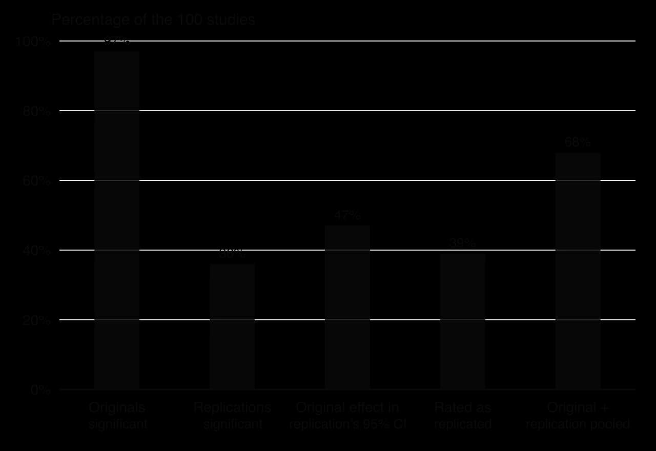
The chart shows that the conclusion does not depend on the measure chosen: between 36% and 47% of findings replicated on the significance, confidence-interval and subjective measures (39% were judged to have replicated by the teams themselves). Combining original and replication data left 68% significant, but this figure assumes that the original results were not inflated by publication bias. Replication rates also differed by field: about half of the cognitive psychology findings replicated, compared with about a quarter of the social psychology findings.
Replication success was better predicted by the strength of the original evidence than by the characteristics of the research teams. Original findings with very small p-values (for example p < 0.001) replicated more often than those with p-values only just below 0.05, and effects that had been judged more surprising tended to replicate less often.
Conclusions
The authors concluded that a large share of published psychological findings were weaker than reported, despite the replications using the original materials and high power. The pattern is consistent with publication bias and flexible analysis favouring significant results, small original samples overestimating effect sizes, and p-values just below 0.05 providing weak evidence. They stressed that a failed replication does not prove an original finding false, and that a successful one does not prove it true, but that the overall rate signalled a problem with how the field produced evidence.
Evaluation
Measurement: what counts as a replication?
The project’s main strength is that it measured replication in five ways and published all its data, so other researchers could check its conclusions. Its main difficulty is that each original study was repeated only once. A single replication with 80–90% power will itself miss a real effect 10–20% of the time, so some “failures” will be type II errors. The 36% figure is therefore an estimate of how often findings replicate on one attempt, not a list of which findings are false.
Bias: were the replications faithful?
Gilbert, King, Pettigrew and Wilson (2016) criticised the project, arguing that some replications differed from the originals in important ways (for example, some were run with different populations or in different countries from the originals) and that, once such differences were taken into account, reproducibility could be quite high. The project’s authors replied that Gilbert et al. had misread the statistics, and that both optimistic and pessimistic readings of the data were possible but neither was yet warranted. The debate shows that changes in sample and culture are a genuine source of variation, which is itself a reason to be careful about generalising a single study.
Causality: why did findings fail to replicate?
The project measured how often findings failed but could not show why. A failure could reflect a false positive in the original, a real effect that is smaller than first reported, or a real effect that depends on conditions (time, place, culture) that differed in the replication. The correlational analysis of what predicted success (strong original evidence, intuitive effects) cannot separate these explanations. Later large projects that tested the same effects in many countries, such as the Many Labs studies, found that some effects replicated almost everywhere while others replicated almost nowhere, which suggests that many failures reflect weak original evidence rather than differences between populations.
Responsibility: what the project changed
By publishing an uncomfortable result about their own field, the authors contributed to reforms that make published findings more trustworthy: pre-registration, Registered Reports, open data and larger samples. The project also raises responsibility questions for how psychology is communicated, since findings from the 2008 literature had already been used in popular books, training programmes and policy before their weakness was known.
Sources: Open Science Collaboration (2015). Estimating the reproducibility of psychological science. _Science, 349(6251), aac4716. Gilbert, D. T., King, G., Pettigrew, S. & Wilson, T. D. (2016). Comment on “Estimating the reproducibility of psychological science”. Science, 351(6277), 1037._
Evaluating significance testing
Null hypothesis significance testing (often shortened to NHST) is still the standard way of drawing conclusions from quantitative data in psychology, and the replication crisis did not end its use. It did make researchers far more aware of what a significance test can and cannot do, and the six concepts provide a useful way to organise its strengths and limitations.
Concept | Strength of significance testing | Limitation of significance testing |
|---|---|---|
Measurement | Gives a shared, objective rule for deciding when a result is unlikely to be due to sampling error. | Reduces evidence to a yes/no decision at an arbitrary cut-off; p depends on sample size, so it measures detectability as much as effect. |
Causality | In a true experiment with random allocation, a significant difference is strong evidence that the IV caused the change in the DV. | Significance cannot show causation in correlational or quasi-experimental data; it says nothing about confounding variables or reverse causation. |
Bias | A fixed α set in advance controls the false-positive rate of an honest, single test. | Publication bias, p-hacking and multiple comparisons can push the real false-positive rate far above 5%. |
Change | Helps judge whether a treatment or intervention had an effect beyond chance. | A significant change may be too small to matter; effect size and practical significance are needed to judge real change. |
Perspective | Fits a positivist, quantitative view of psychology that values replication and hypothesis testing. | Says nothing about meaning or experience; qualitative methods such as thematic analysis answer different questions. |
Responsibility | Transparent reporting allows others to check and repeat analyses. | Over-claiming from p-values can mislead the public and policy-makers; uncertainty has to be communicated honestly. |
Alternatives and additions
Most statisticians now recommend reporting estimates alongside or instead of p-values: the effect size with its confidence interval shows how large an effect is and how precisely it has been measured. Bayesian statistics offer a different approach, in which the strength of evidence for one hypothesis over another (a Bayes factor) is calculated directly, so that data can support the null hypothesis rather than only fail to reject it. Meta-analysis, which combines effect sizes from many studies, reduces dependence on any single p-value, although it is only as good as the studies it includes and can be distorted by publication bias.
Culture and generalisation
A significant result says nothing about whether an effect holds in other cultures. Much of the research in the replication debates used samples from North America and Europe, often university students, so even a well-replicated effect may be limited to WEIRD samples. Multi-site projects that test the same procedure in many countries help in two ways: they provide high power and show whether an effect varies across cultures. A finding that replicates in samples from Asia, Africa, Latin America and Europe is far stronger evidence than a significant result from one laboratory.
Exam practice
Inferential statistics appear in Paper 3, where a booklet of four to six unseen sources is built around a claim about culture, motivation or technology in one of the four contexts. Questions 1 and 2 often turn on reading inferential statistics: spotting what limits the interpretation of a result, and analysing descriptive and inferential findings to reach a conclusion about the claim. Questions ask for interpretation, not calculation.
The practice items share one invented source booklet. Claim: the use of smartphones in class has a negative effect on students’ learning. All data are hypothetical.
Source 1. A bar graph shows mean scores on a 20-item quiz: “phone on desk” 13.1, “phone in bag” 14.0. The y-axis runs from 12 to 14.5. No sample size, standard deviations or test result are given.
Source 2. An experiment at two secondary schools randomly allocated 120 students (aged 15–16) to attend a lecture with their phone on the desk or left outside the room, then tested recall the next day.
Outcome | Phone on desk (n = 60) | Phone outside (n = 60) | Test result | Effect size (d) |
|---|---|---|---|---|
Recall of lecture content (out of 30) | M = 17.9, SD = 4.6 | M = 19.8, SD = 4.4 | t(118) = 2.31, p = 0.023 (two-tailed) | 0.42 |
Self-rated concentration (1–7) | M = 4.6, SD = 1.2 | M = 4.9, SD = 1.1 | t(118) = 1.43, p = 0.155 (two-tailed) | 0.26 |
Self-rated enjoyment of lecture (1–7) | M = 5.0, SD = 1.3 | M = 4.9, SD = 1.4 | t(118) = 0.41, p = 0.684 (two-tailed) | 0.07 |
Source 3. A researcher who teaches at one of the schools interviewed eight teachers about phones in lessons. Extract: “They say they only check the time, but you can see the attention drain away… I think the ones who struggle most are the ones who can’t leave it alone.” The researcher concludes that phones harm learning, especially for weaker students.
Question 1 rewards an issue that is identified, described and then explained in relation to the claim. Naming two issues adds nothing; explaining one well earns all three marks.
Question 4 asks for a judgement on the whole claim. The top band needs at least three sources interpreted with own knowledge, different points of view evaluated and a reasoned conclusion, so a plan organised source by source, each linked back to the claim, works well.
Summary
Inferential statistics judge whether a difference or relationship in a sample is likely to reflect the population or could easily be due to sampling error.
A test assumes the null hypothesis (no effect) is true; the p-value is the probability of results at least this extreme if it is, not the probability that it is true.
If p ≤ α (usually 0.05) the result is significant and the null hypothesis is rejected; otherwise it is retained, which is not proof of no effect.
One-tailed tests put the whole 5% in the predicted direction and must be chosen in advance; two-tailed tests split it between both tails.
A type I error is a false positive (probability α); a type II error is a false negative (probability β). Lowering α reduces one and raises the other.
Statistical power rises with sample size and effect size; underpowered studies miss real effects and exaggerate the effects they do find.
Statistical significance is not practical significance: effect sizes such as Cohen’s d and confidence intervals show how large and precise an effect is.
Multiple comparisons and p-hacking push the real false-positive rate far above 5%, as the dead salmon and “When I’m Sixty-Four” studies showed.
The Open Science Collaboration (2015) found that only 36% of 100 replications were significant, against 97% of originals, with effects about half as large.
Pre-registration, Registered Reports, open data and large multi-site replications are the main reforms that followed the replication crisis.
Self-check
- To do:
I can explain why psychologists use inferential statistics and how they differ from descriptive statistics.
- To do:
I can describe the logic of a significance test using the null and alternative hypotheses, the significance level and the p-value.
- To do:
I can interpret a reported test result, including whether it was one- or two-tailed, and word the conclusion correctly.
- To do:
I can explain type I and type II errors and the trade-off between them.
- To do:
I can explain how sample size and statistical power affect what a study can conclude.
- To do:
I can compare and contrast statistical and practical significance, using effect size and confidence intervals.
- To do:
I can explain how multiple comparisons and p-hacking produce false positives and how they contributed to the replication crisis.
- To do:
I can evaluate significance testing with reference to measurement, bias and causality.
- To do:
I can analyse inferential statistics in an unfamiliar source and state a conclusion linked to a claim.