12.2 Descriptive statistics

Calculate and interpret measures of central tendency and dispersion, percentages and correlation coefficients, and use them to analyse research findings and draw conclusions that are linked to the data.

IB Psychology
Part of 12 Data analysis and interpretation
HL only

Key terms introduced here

Each is in the Psychology glossary, with every other term in the subject.

Coefficient of determination: The square of the correlation coefficient (r²), which gives the proportion of the variation in one variable that is accounted for by its linear relationship with the other.
Interquartile range: A measure of dispersion: the difference between the upper quartile and the lower quartile, giving the spread of the middle 50% of scores; it is not affected by extreme scores.
Measure of dispersion: A descriptive statistic that shows how spread out the scores in a data set are, such as the range, the interquartile range or the standard deviation.
Range: A measure of dispersion: the difference between the highest and lowest scores in a data set. It is quick to calculate but depends entirely on the two most extreme scores.
Standard deviation: A measure of dispersion that shows how far, on average, scores lie from the mean of their data set. A small standard deviation means scores cluster closely around the mean.
Variance: A measure of dispersion equal to the average of the squared deviations of scores from their mean; its square root is the standard deviation.
z-score: A score expressed as the number of standard deviations it lies above or below the mean of its distribution, which allows scores from different tests to be compared.

Carry on with 12.2 in Augment

With a free account, Augment remembers where you stopped and what you have practiced.

Start free Open 12.2 in Augment

12.2 Descriptive statistics · IB Psychology | Augment Education

12.2 Descriptive statistics

IB Psychology
Part of 12 Data analysis and interpretation
HL only

Key terms introduced here

Each is in the Psychology glossary, with every other term in the subject.

Coefficient of determination: The square of the correlation coefficient (r²), which gives the proportion of the variation in one variable that is accounted for by its linear relationship with the other.
Interquartile range: A measure of dispersion: the difference between the upper quartile and the lower quartile, giving the spread of the middle 50% of scores; it is not affected by extreme scores.
Measure of dispersion: A descriptive statistic that shows how spread out the scores in a data set are, such as the range, the interquartile range or the standard deviation.
Range: A measure of dispersion: the difference between the highest and lowest scores in a data set. It is quick to calculate but depends entirely on the two most extreme scores.
Standard deviation: A measure of dispersion that shows how far, on average, scores lie from the mean of their data set. A small standard deviation means scores cluster closely around the mean.
Variance: A measure of dispersion equal to the average of the squared deviations of scores from their mean; its square root is the standard deviation.
z-score: A score expressed as the number of standard deviations it lies above or below the mean of its distribution, which allows scores from different tests to be compared.

Carry on with 12.2 in Augment

With a free account, Augment remembers where you stopped and what you have practiced.

Start free Open 12.2 in Augment

Notes on 12.2 Descriptive statistics

34 min readLast reviewed 15 Oct 2026

Learning objectives

Describe the purpose of descriptive statistics and how they differ from inferential statistics.
Explain when the mean, median and mode are each the most appropriate measure of central tendency.
Interpret the range, interquartile range and standard deviation of a set of scores, and explain how each is calculated.
Interpret percentages, proportions and z-scores, including the base numbers behind them.
Interpret a correlation coefficient and the coefficient of determination (r²) as descriptive statistics.
Analyse descriptive statistics in a source by comparing centre and spread, considering sample size, and stating a conclusion linked to the findings.
Evaluate the use of descriptive statistics in research with reference to measurement, bias and causality.

Introduction

Descriptive statistics summarise a set of data with a few numbers: an average that shows the typical score, a measure of how spread out the scores are, and, for two variables, a measure of how closely they are related. They are the first thing a researcher calculates and the first thing a reader checks, because every later conclusion rests on them.

Descriptive statistics can clarify a finding or distort it. A mean without a measure of spread can make a small difference look important; a percentage without its base number can make a rare event look common. Reading them critically draws on the concept of measurement (what exactly was counted or scored), bias (which statistics a researcher chose to report) and causality (what a difference or correlation can and cannot show).

What descriptive statistics do

A study with 60 participants produces 60 scores in each condition. Nobody can compare two lists of 60 numbers by eye, so researchers summarise each list. Descriptive statistics describe the data that were actually collected: the participants in the sample, measured in the way the study measured them. They do not, on their own, say whether the pattern would be found again or in the wider target population.

That second question belongs to inferential statistics, which estimate how likely it is that a difference or relationship in the sample reflects a real effect rather than chance. The two work together: descriptive statistics show the size and direction of a pattern, and inferential statistics judge whether it is likely to be more than chance. A result can be statistically significant but tiny, or large but uncertain, so a full interpretation always needs the descriptive numbers.

Kind of descriptive statistic	Question it answers	Main examples
Measure of central tendency	What is a typical score?	Mean, median, mode
Measure of dispersion	How spread out are the scores?	Range, interquartile range, standard deviation
Proportions	How common is something?	Percentages, proportions, rates per 100,000
Measures of relationship	How closely do two variables go together?	Correlation coefficient (r), coefficient of determination (r²)

Measures of central tendency

A measure of central tendency gives one value that represents the centre or typical point of a set of scores. There are three, and each defines “typical” differently. Choosing between them is a decision about the level of measurement and the shape of the distribution.

The mean

The mean is the arithmetic average: the sum of all the scores divided by the number of scores. It is written $\bar{x}$ (“x bar”) for a sample.

\bar{x} = \frac{\sum x}{n}

Here $\sum x$ means “add up every score” and $n$ is the number of scores. For the recall scores 6, 8, 9, 9 and 13, the sum is 45 and $n$ = 5, so the mean is 9 words.

The mean uses every score, which makes it the most sensitive average and the basis of most further statistics, including the standard deviation. The same property is its weakness: one extreme score pulls it towards itself. Rosenhan’s pseudo-patients, for example, stayed in hospital for between 7 and 52 days; a single very long stay raises the mean length of stay much more than it raises the median. The mean suits interval or ratio data that are roughly symmetrical.

The median

The median is the middle score when all the scores are placed in order. With an odd number of scores it is the one in the middle; with an even number it is halfway between the two middle scores. For 4, 5, 5, 6, 6, 7 and 42, the median is 6. For 3, 5, 8 and 10, it is (5 + 8) ÷ 2 = 6.5.

Because the median depends only on the order of the scores, the value of the extreme scores does not matter. If 42 became 420, the median would still be 6. This makes the median the better average for skewed data, data with outliers and ordinal data such as rankings or ratings. Its weakness is that it ignores most of the information in the data: two very different sets of scores can have the same median.

The mode

The mode is the score or category that occurs most often. It is the only average that can be used with nominal data: the modal attachment type in a sample, or the most common answer to a multiple-choice question. A set of data can have no mode (every score occurs once), one mode, or two (bimodal) or more. The mode is easy to find but unstable in small samples, where a single score can change it.

Choosing the right average

Average	Uses	Strengths	Limitations
Mean	Interval or ratio data, roughly symmetrical, no extreme outliers	Uses every score; basis for the standard deviation and most inferential tests	Distorted by outliers and skew; may be a value nobody scored (2.4 children)
Median	Ordinal data; skewed interval or ratio data; data with outliers	Not affected by extreme scores; easy to understand as “the middle person”	Ignores the values of most scores; less useful for further calculation
Mode	Nominal data; the most common category or score	The only average for categories; shows the most typical response	May not exist or may be several values; unstable in small samples

In a symmetrical distribution the three averages are close together, and the mean is usually reported. In a skewed distribution they separate, with the mean pulled towards the long tail, so the gap between the mean and the median is itself a useful clue: when the mean is much larger than the median, the data are probably positively skewed or contain high outliers.

CrashCourse Statistics: the mean, median and mode, and why skewed data and outliers make the choice between them matter.

Measures of dispersion

Two groups can have exactly the same mean and be completely different. In one, every participant may score close to the mean; in the other, half may score very high and half very low. A measure of dispersion describes how spread out the scores are, and it is needed to judge whether the difference between two averages is large or small compared with the differences between individuals.

The range

The range is the difference between the highest and the lowest score. For the scores 4, 5, 5, 6, 6, 7 and 42, the range is 42 − 4 = 38. Some textbooks add 1 to allow for rounding of measurements, but the simple difference is the more common definition.

The range is easy to calculate and to understand, but it is based on only two scores. One outlier can make it very large, as the score of 42 does here, while the other six scores lie within 3 points of each other. The range is therefore a rough first look, and it is usually reported with another measure.

The interquartile range

The interquartile range (IQR) is the range of the middle 50% of the scores: the upper quartile (Q3) minus the lower quartile (Q1). Because it ignores the lowest quarter and the highest quarter of the data, it is not affected by extreme scores, which makes it the natural partner of the median.

For a small data set, the quartiles can be found by splitting the ordered scores in half at the median and finding the median of each half. Statistical software uses slightly different formulas, so published quartiles can differ a little from hand calculations, but the idea is the same.

Calculate the interquartile range of these reaction times (milliseconds) from 10 participants: 310, 280, 450, 330, 295, 360, 305, 345, 320, 900 (hypothetical data).

Show the solution

Step 1: order the scores. 280, 295, 305, 310, 320, 330, 345, 360, 450, 900.

Step 2: find the median. With 10 scores, the median lies between the 5th and 6th: (320 + 330) ÷ 2 = 325 ms.

Step 3: split into halves. Lower half: 280, 295, 305, 310, 320. Upper half: 330, 345, 360, 450, 900.

Step 4: find the quartiles. Q1 is the median of the lower half, 305 ms. Q3 is the median of the upper half, 360 ms.

Step 5: subtract. IQR = 360 − 305 = 55 ms. By contrast, the range is 900 − 280 = 620 ms, inflated by the single score of 900, which may be a participant who was distracted. The IQR describes the spread of the typical participants far better.

The standard deviation

The standard deviation (SD) measures the typical distance of the scores from their mean. If most scores are close to the mean, the standard deviation is small; if they are widely scattered, it is large. Unlike the range and the IQR, it uses every score, so it is the most informative measure of spread for interval or ratio data that are roughly normal. It is always reported with the mean (for example, “M = 12.4, SD = 3.1”).

How it is calculated

The calculation follows directly from the idea of “distance from the mean”. Each score’s deviation from the mean is found and squared (so that negative and positive deviations do not cancel out). The squares are added and divided by $n - 1$ , which gives the variance. The square root of the variance brings the result back to the original units.

s = \sqrt{\frac{\sum (x - \bar{x})^2}{n - 1}}

Dividing by $n - 1$ rather than $n$ is a correction used when the data are a sample: a sample’s scores tend to lie slightly closer to their own mean than to the population mean, so dividing by $n - 1$ makes the estimate a little larger and more accurate. Most calculators and software do this automatically.

Five participants recall 4, 6, 7, 8 and 10 words. Calculate the standard deviation.

Show the solution

Step 1: find the mean. (4 + 6 + 7 + 8 + 10) ÷ 5 = 35 ÷ 5 = 7.

Score (x)	Deviation (x − 7)	Squared deviation
4	−3	9
6	−1	1
7	0	0
8	1	1
10	3	9
	Sum of deviations = 0	Sum of squares = 20

Step 2: divide by n − 1. 20 ÷ 4 = 5. This is the variance.

s = \sqrt{5} \approx 2.24 \text{ words}

Interpreting the standard deviation

A standard deviation is meaningful only in relation to its mean and its scale. An SD of 2 words in a recall test with a mean of 7 shows considerable variation (most participants fall between about 5 and 9), whereas an SD of 2 points on an IQ test would be extremely small. Comparing SDs across conditions shows whether a manipulation made people more alike or more varied: a treatment that lowers the mean anxiety score and also halves its SD has produced a more consistent effect.

When data are roughly normal, the standard deviation also describes the shape of the distribution. About 68% of scores fall within one SD of the mean, about 95% within two, and about 99.7% within three. On intelligence tests standardised with a mean of 100 and an SD of 15, about 68% of people score between 85 and 115 and about 95% between 70 and 130.

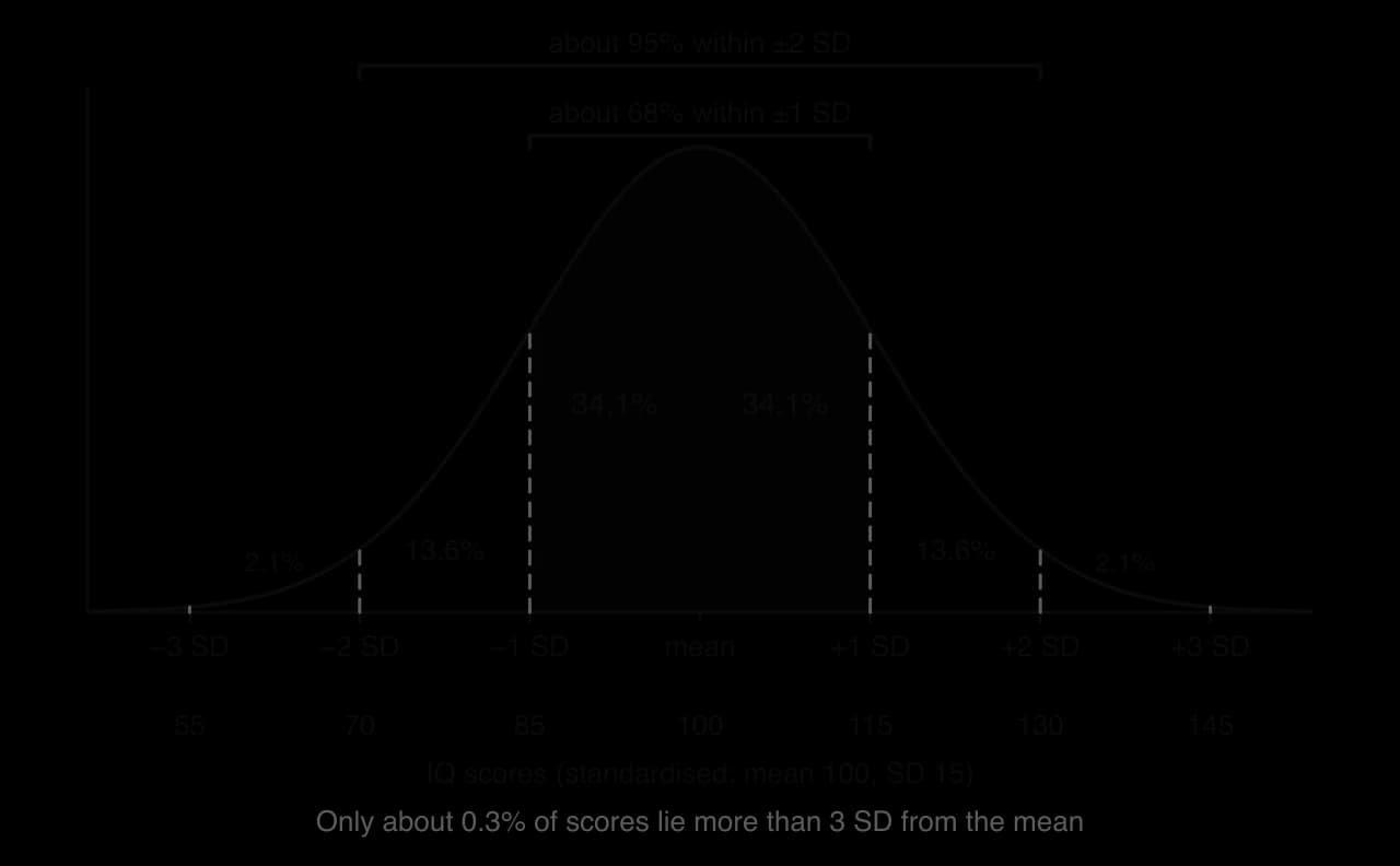
Normal curve divided at each standard deviation: 34.1% of scores between the mean and 1 SD on each side, 13.6% between 1 and 2 SD, 2.1% between 2 and 3 SD; about 68% within ±1 SD, 95% within ±2 SD. IQ scale: 55, 70, 85, 100, 115, 130, 145. — For normal data, the SD fixes the proportion of scores in each band, so a mean and SD together describe the whole distribution. IQ tests are scaled so that 1 SD = 15 points.

The same mean can sit inside very different spreads. Two groups with a mean of zero, one with an SD of 1 and one with an SD of 2, share their centre but not their shape: the second is flatter and wider, with many more extreme scores.

A z-score expresses an individual score as the number of standard deviations it lies from the mean: $z = (x - \bar{x}) \div s$ . An IQ of 130 is $z$ = (130 − 100) ÷ 15 = +2, which on a normal distribution places the person above about 97.7% of the population. Z-scores allow scores from different tests to be compared, which is why researchers who use several tests of different difficulty often convert scores to z-scores before combining them.

CrashCourse Statistics: the range, interquartile range, variance and standard deviation, and what each says about spread.

Measure of dispersion	Best used with	Strength	Limitation
Range	A quick look at any ordinal, interval or ratio data	Simple; shows the full span	Depends only on the two extreme scores
Interquartile range	Skewed data or data with outliers; reported with the median	Not affected by extreme scores	Ignores half of the data
Standard deviation	Roughly normal interval or ratio data; reported with the mean	Uses every score; links to the normal curve and to inferential tests	Inflated by outliers and skew; harder to calculate by hand

Percentages and proportions

Many psychological findings are reported as percentages: the proportion of participants who conformed, who reported a false memory, or who met the criteria for a disorder. A percentage is a count divided by a base and multiplied by 100. A proportion is the same value as a decimal (0.32 rather than 32%). Rates per 100,000 people, used for suicide or disease statistics, are another form of proportion that makes small numbers easier to compare between populations of different size.

Every percentage depends on its base. “Half of the participants improved” means something very different when there were 4 participants than when there were 4,000, and when the comparison group improved at a similar rate. Three distinctions prevent most errors:

Percentage points versus per cent. A rise from 10% to 15% is an increase of 5 percentage points but a 50% relative increase. Reports that say “a 50% rise” without the starting value can make a small change sound large.
Absolute versus relative differences. If a condition affects 2 in 1,000 people in one group and 4 in 1,000 in another, the relative risk has doubled, but the absolute difference is 2 people per 1,000.
The right denominator. “40% of people with depression use social media heavily” is not the same as “40% of heavy social media users have depression”. The two percentages use different bases and can be very different numbers.

In a hypothetical study, 18 of 60 students who used a revision app (30%) and 9 of 45 students who did not (20%) reported feeling “very confident” before a test. A school newsletter says: “The app makes students 50% more confident.” Interpret these figures.

Show the solution

Step 1: check the bases. 18 ÷ 60 = 30% and 9 ÷ 45 = 20%. The groups differ in size, so comparing the percentages, not the counts, is correct.

Step 2: separate absolute and relative differences. The absolute difference is 10 percentage points. The relative difference is 10 ÷ 20 = 50%, which is where the newsletter’s figure comes from. Both are accurate, but “50% more confident” sounds much larger than “10 percentage points”.

Step 3: check the measure and the design. “Very confident” is one self-report category, not a measure of confidence across all students, and the students chose whether to use the app, so more confident students may simply have been more likely to use it.

Step 4: conclude. The data show a modest difference in the proportion of very confident students; they cannot show that the app causes greater confidence.

The correlation coefficient as a descriptive statistic

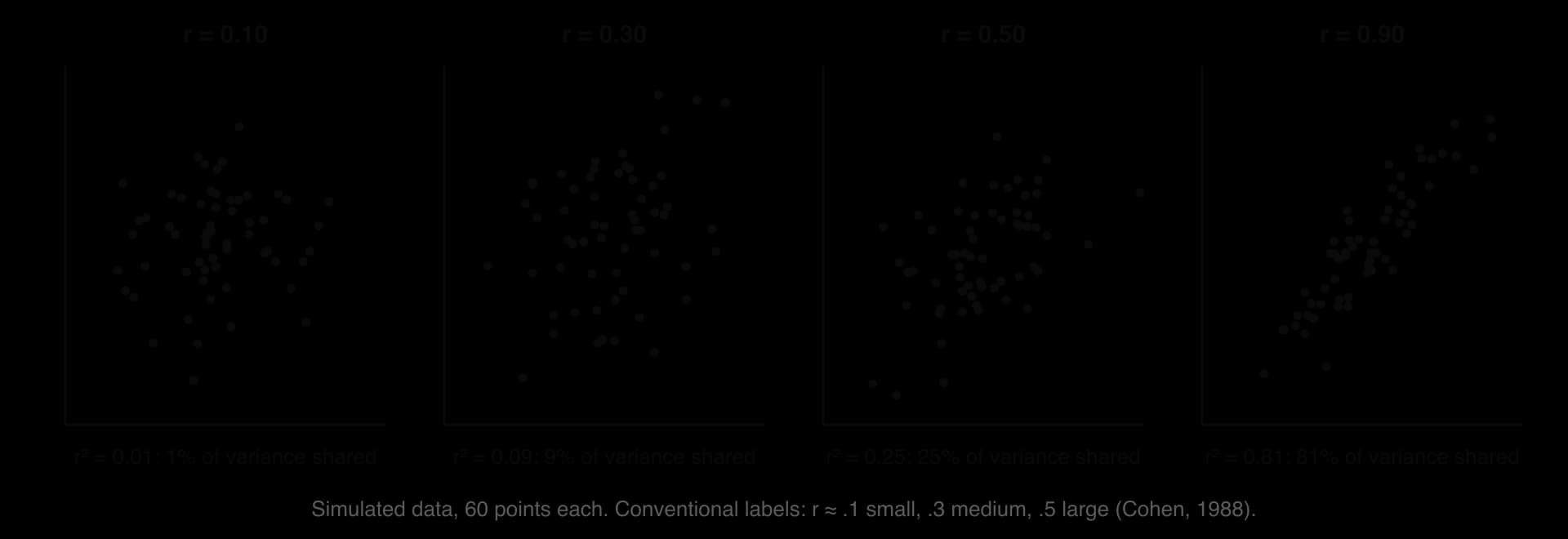
When a study measures two variables in the same participants, the correlation coefficient (r) describes how closely they are related. It runs from −1 (a perfect negative relationship) through 0 (no linear relationship) to +1 (a perfect positive relationship). The sign gives the direction and the size, ignoring the sign, gives the strength. A correlation of −0.45 is therefore stronger than one of +0.30.

Strength is often described using conventions proposed by the statistician Jacob Cohen (1988): about .10 is small, about .30 medium and about .50 or above large. These are rough guides for research in the behavioural sciences, not rules. In psychology, correlations above .50 between different variables are uncommon, and a correlation of .30 can matter a great deal if the outcome is important.

Four simulated scatterplots of 60 points: r = 0.10 (shapeless cloud, r² 1%), r = 0.30 (faint upward tilt, 9%), r = 0.50 (clear upward trend, 25%) and r = 0.90 (tight line, 81%). — A correlation of .30, a typical “medium” effect in psychology, is hard to see by eye; only near .90 do the points form a clear line. r² gives the share of variance the two variables have in common.

The coefficient of determination (r²)

Squaring the correlation coefficient gives the coefficient of determination (_r_²), the proportion of the variation in one variable that is accounted for by its linear relationship with the other. A correlation of .50 gives _r_² = .25: 25% of the variation in one variable is shared with the other, and 75% is not. Because squaring a number smaller than 1 makes it smaller, _r_² shows how modest many apparently respectable correlations are.

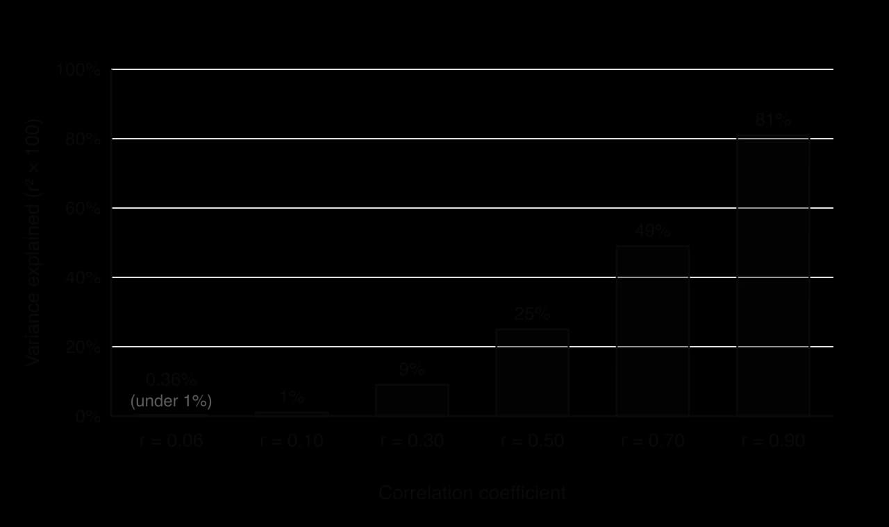
Bar chart of variance explained (r squared as a percentage) for correlations of 0.06 (0.36%), 0.10 (1%), 0.30 (9%), 0.50 (25%), 0.70 (49%) and 0.90 (81%). — Variance explained grows with the square of r: doubling r from .3 to .6 quadruples r², and correlations below about .1 explain less than 1% of the variation.

Orben and Przybylski (2019) used this idea in a debate about adolescents and digital technology. Analysing three large data sets with 355,358 adolescents in total, and testing many reasonable ways of analysing them, they found that the association between technology use and well-being was negative but small: technology use explained at most 0.4% of the variation in well-being, equivalent to a correlation of about .06. With samples this large, such a small correlation can be statistically significant, so _r_² is a useful reminder of how little of the variation it accounts for.

The correlation coefficient describes association, not causation. Even a large r is compatible with either variable affecting the other (bidirectional ambiguity) or with a third variable affecting both. It also measures only straight-line relationships: a strong curved relationship can give r close to zero, and a single outlier can create or destroy a correlation, which is why a scatterplot should always be checked.

Effect sizes for differences between means

A correlation coefficient is one kind of effect size: a number that describes how large a relationship or difference is, independent of sample size. For a difference between two means, the most common effect size is Cohen’s d, the difference between the means divided by the (pooled) standard deviation. A d of 0.5 means the two means are half a standard deviation apart. Cohen’s conventions for d are 0.2 small, 0.5 medium and 0.8 large. Effect sizes link the two halves of this subtopic: they combine a measure of central tendency (the difference between means) with a measure of dispersion (the standard deviation) in one number.

d = \frac{\bar{x}_1 - \bar{x}_2}{s_{\text{pooled}}}

Choosing and reporting descriptive statistics

The choice of statistics follows from the level of measurement and the shape of the data. Researchers usually report a measure of central tendency and a measure of dispersion that belong together: the mean with the standard deviation, or the median with the interquartile range. Reporting a mean with no measure of spread, or a percentage with no base number, leaves the reader unable to judge the result.

Flow chart: nominal data → mode, frequencies and percentages; ordinal data → median with range or interquartile range; interval or ratio data → mean and SD if roughly symmetrical with no extreme outliers, otherwise median and IQR. — The level of measurement narrows the choice, and the shape of the distribution settles it: skew or outliers point to the median and IQR, symmetrical data to the mean and SD.

Analysing descriptive statistics in a source

Interpreting descriptive statistics follows the same steps whatever the study. The aim is to turn the numbers into an accurate description and then into a conclusion that goes no further than the numbers allow.

Identify what was measured, in whom. Name the variables, the units or scale, the groups or conditions and the sample size.
Describe the centre with numbers. State the means or medians, which is highest, and the size of the difference (in units and, where useful, as a percentage of the scale).
Describe the spread. Compare the SDs or IQRs. Large spreads relative to the difference mean the groups overlap heavily; a smaller spread in one group means it was more consistent.
Look for distortion. Check for skew (mean far from median), outliers, small or unequal groups, floor or ceiling effects, and percentages without bases.
Consider the design. Was there random allocation? If not, a difference or correlation may reflect other variables.
State a cautious conclusion linked to the numbers. Use wording such as “suggests”, “is consistent with” or “provides limited support for”, and name the specific findings it rests on.

A hypothetical study gives 30 students a vocabulary test after learning with spaced practice and 30 after massed practice (cramming). Spaced: M = 34.0, SD = 4.2, median = 34. Massed: M = 29.5, SD = 9.8, median = 32. Scores are out of 40. Analyse these results.

Show the solution

Step 1: centre. The spaced group scored higher on average: a mean of 34.0 compared with 29.5, a difference of 4.5 marks (about 11% of the 40-mark test).

Step 2: spread. The massed group’s SD (9.8) is more than twice that of the spaced group (4.2), so the massed students varied much more: some did as well as the spaced group and some did much worse.

Step 3: distortion. In the massed group, the mean (29.5) is well below the median (32), which suggests negative skew: a few very low scores are pulling the mean down. Comparing medians, the difference shrinks to 2 marks. The spaced group’s mean and median are the same (34), which suggests a symmetrical distribution, and its scores may be near the test’s ceiling of 40.

Step 4: conclusion. The results suggest that spaced practice led to higher and more consistent scores, but part of the difference in means comes from a few low scorers in the massed group. With 30 students per group and large overlap, an inferential test and an effect size would be needed to judge how reliable the difference is.

Evaluating descriptive statistics

Measurement: a summary is only as good as the measure behind it

A mean of 4.2 on a five-point “happiness” scale summarises responses to particular questions, not happiness itself. Descriptive statistics inherit every weakness of the measure: social desirability in self-report, floor and ceiling effects, and ordinal scales treated as interval data. They also hide individuals. A mean improvement after therapy can hide some participants who got worse, which is why researchers in clinical psychology also report how many individuals improved, stayed the same or deteriorated.

Bias: which statistics are reported

Researchers decide which statistics to calculate and which to report. Reporting the mean when the median would tell a less impressive story, choosing a relative rather than absolute percentage, or leaving out standard deviations can all make a finding look stronger than it is, even when every number is accurate. Open data, in which the raw scores are published, lets others check whether the summary is fair.

Causality: descriptions are not explanations

A difference between means or a correlation describes a pattern; it does not explain it. Whether the pattern reflects a causal effect depends on the design (random allocation, controls), not on the size of the statistic. Large differences between groups that were not randomly allocated, such as people who choose a particular app, school or therapy, may reflect who chose rather than what was chosen.

Culture and perspective

Descriptive statistics from one population may not describe another. Response styles differ between cultures: some studies find that participants in East Asian samples use the middle of rating scales more than participants in North American samples, which can lower means and SDs for reasons that have nothing to do with the construct being measured. Comparing means across cultures therefore requires evidence that the measure works in the same way in each group.

Concept	Question to ask of any descriptive statistic
Measurement	What exactly was scored or counted, on what scale, and could the scale have a floor or ceiling?
Bias	Which statistics are missing (spread, base numbers, medians), and would they change the picture?
Causality	Was there random allocation, or could the difference or correlation reflect other variables?
Perspective	Does the average describe every group in the sample, or are subgroups or cultures hidden inside it?

Key study: Mueller and Oppenheimer (2014) and its replication

The claim that taking notes by hand is better for learning than taking them on a laptop is widely repeated in schools and universities. The original study and a later direct replication show how descriptive statistics, read carefully, can support one part of a conclusion and not another.

Aim

Pam Mueller and Daniel Oppenheimer aimed to find out whether taking lecture notes on a laptop rather than by hand affects learning, and whether any effect could be explained by laptop users copying the lecture word for word (verbatim) instead of processing it into their own words.

Method

In Study 1, 67 students from the Princeton University participant pool took part (two were later excluded, one because he had already seen the lecture and one because of a recording error). It was a true experiment with an independent samples design: participants were allocated to take notes either on a laptop disconnected from the internet or in a notebook. They watched one of five TED talks, each about 15 minutes long, and were told to take notes as they normally would in class.

Participants then completed several distractor tasks, including a demanding working-memory task, before answering two kinds of question about the talk: factual-recall questions (such as approximately how many years ago a civilisation existed) and conceptual-application questions (such as how two countries differed in their approach to equality). Because the five talks differed in difficulty, scores were converted to z-scores. The notes were analysed for the number of words and for verbatim overlap, measured as the percentage of three-word sequences that matched the lecture transcript.

Results

On factual questions, the two groups performed almost identically (laptop M = 0.021, SD = 1.31; longhand M = 0.009, SD = 1.02). On conceptual questions, laptop users scored lower (M = −0.156, SD = 0.915) than longhand users (M = 0.154, SD = 1.08), a statistically significant difference. Laptop notes contained far more words (M = 309.6, SD = 116.5, against 173.4, SD = 70.7; d = 1.4) and more verbatim overlap (14.6%, SD = 7.3%, against 8.8%, SD = 4.8%; d = 0.94).

Three bar charts with ±1 SD error bars. Words: laptop 309.6 (SD 116.5), longhand 173.4 (SD 70.7). Verbatim overlap: 14.6% (SD 7.3) vs 8.8% (SD 4.8). Quiz z-scores: factual 0.021 vs 0.009; conceptual −0.156 vs 0.154; SDs about 0.9–1.3. — The differences in the notes are large compared with their SDs; the conceptual quiz difference (0.31 SD) is small compared with SDs near 1, so the groups overlap heavily. Source: Mueller & Oppenheimer (2014), Study 1.

Two further studies extended the result. In Study 2 (151 students), telling laptop users not to copy the lecture word for word did not reduce their verbatim overlap, and longhand note-takers again did better on conceptual questions. In Study 3 (109 students), participants returned a week later; those who had taken longhand notes and were allowed to review them generally performed best.

Conclusions

Mueller and Oppenheimer concluded that laptop note-taking leads to shallower processing: because typing is fast, laptop users transcribe more of the lecture verbatim, and this verbatim note-taking harms conceptual understanding. Their recommendation, that laptops in lectures may do more harm than good, was widely reported and used to justify classroom laptop bans.

The replication: Urry et al. (2021)

Heather Urry and colleagues at Tufts University carried out a direct replication of Study 1, following the original procedure as closely as possible, with 142 students (74 laptop, 68 longhand). The note-taking results replicated: laptop users again wrote more words and copied more of the lecture verbatim. The learning result did not: the laptop and longhand groups did not differ in quiz performance. A mini meta-analysis of eight similar studies, including the original, showed the same pattern, with clear differences in the notes but no reliable difference in performance. In both the original and the replication, writing more words went with better quiz scores.

Finding	Mueller & Oppenheimer (2014), Study 1	Urry et al. (2021) replication
Sample	67 Princeton students (2 excluded)	142 students (74 laptop, 68 longhand)
Words written	Laptop much higher (309.6 vs 173.4; d = 1.4)	Laptop higher (replicated)
Verbatim overlap	Laptop higher (14.6% vs 8.8%; d = 0.94)	Laptop higher (replicated)
Factual quiz	No difference	No difference
Conceptual quiz	Longhand higher (z = 0.154 vs −0.156)	No reliable difference (not replicated)

Sources: Mueller, P. A., & Oppenheimer, D. M. (2014). The pen is mightier than the keyboard: Advantages of longhand over laptop note taking. _Psychological Science, 25(6), 1159–1168. Urry, H. L., et al. (2021). Don’t ditch the laptop just yet: A direct replication of Mueller and Oppenheimer’s (2014) Study 1 plus mini meta-analyses across similar studies. Psychological Science, 32(3), 326–339._

Evaluation

Measurement: what the descriptive statistics actually show

Reading the original numbers closely explains much of the later dispute. The effects on the notes were large: a d of 1.4 for word count means the average laptop user wrote more than about 92% of longhand writers would be expected to. The effect on conceptual learning was much smaller: a difference of about 0.31 in z-scores, against standard deviations close to 1, means the two distributions overlapped heavily. A large, reliable difference in one measure and a small, fragile difference in another can both be true of the same study, and the replication confirmed exactly the large one.

Measurement choices add uncertainty. The quizzes contained only a few questions per talk, scored by hand (the original reported good agreement between two raters), and z-scores from five different talks were combined. Verbatim overlap was measured mechanically as matching three-word strings, which captures copying but not the quality of the notes. The meta-analysis also found that writing more, which laptops make easier, goes with better scores, which points in the opposite direction from the original recommendation.

Bias: sample size and publication

Study 1 had about 30 participants per condition, and small samples produce unstable means and inflated effect sizes when a result happens to reach significance. A striking, significant result in a small study is more likely to be published and widely reported than a null result, which is one route by which publication bias can shape what teachers and students believe. Morehead, Dunlosky and Rawson (2019) also failed to find a consistent longhand advantage in their own replication and extension.

Generalisability and change

All of these studies used university students, mostly in the United States, watching short recorded talks and tested after about half an hour without the chance to review their notes. Real lectures are longer, students revise from their notes later, and laptop use in class also brings distractions such as messaging, which these studies removed by disconnecting the internet. Typing and handwriting habits also differ across generations and education systems, so the results may change as note-taking habits change.

Exam practice

Descriptive statistics appear in almost every Paper 3 source. Question 2 asks for an analysis of a source’s findings and a conclusion linked to the claim, and that analysis is mainly an analysis of descriptive statistics: means, spreads, percentages and correlations, read alongside the sample and the design. The same skills support Question 1 (an issue that limits interpretation, such as a missing SD) and the synthesis essay.

Practice resource booklet (hypothetical data). The sources have been collated to assess the claim that intrinsic motivation improves long-term retention.

Source 1. A true experiment with 48 university students in one country. Participants learned 30 facts about astronomy either for their own interest (intrinsic condition, told “learn what you find interesting”) or for a reward of €5 for each 10 facts recalled (extrinsic condition). Recall one week later: intrinsic M = 17.2, SD = 3.1, median = 17; extrinsic M = 15.8, SD = 6.4, median = 18.
Source 2. A survey of 1,200 secondary students in three countries. Self-reported intrinsic motivation for science correlated with end-of-year science grades: r = 0.28 overall (country A r = 0.35, country B r = 0.31, country C r = 0.08).
Source 3. Interviews with 12 teachers about how they motivate students, analysed using thematic analysis.

An analysis question builds on the same reading of the numbers but goes further, comparing groups and linking the pattern to the claim.

Question 2 [6 marks]. Analyse the findings from Source 2 and state a conclusion linked to the claim that intrinsic motivation improves long-term retention.

Show a model answer

Step 1: describe the overall relationship. There is a positive correlation of r = 0.28 between intrinsic motivation and science grades: students reporting more intrinsic motivation tend to have higher grades. This is a small-to-medium correlation; _r_² = 0.08, so motivation shares only about 8% of the variation in grades.

Step 2: compare subgroups. The correlation is similar in countries A (0.35, about 12% shared variation) and B (0.31, about 10%) but almost absent in country C (0.08, under 1%). The overall figure therefore hides a cultural difference: the relationship does not hold equally across the three countries.

Step 3: consider measures and design. Motivation is self-reported, and grades are a measure of achievement over a year rather than long-term retention. The design is correlational, so higher grades could increase interest in science as much as interest could raise grades.

Step 4: conclusion. Source 2 provides limited support for the claim: intrinsic motivation is modestly associated with higher grades in two of three countries, but the weak overall relationship, the absence of a relationship in country C, the correlational design and the use of grades rather than retention mean it cannot show that intrinsic motivation improves long-term retention.

Question 3 [6 marks]. Discuss how the researcher could avoid bias in Source 3.

Show an answer plan

Answer plan.

Researcher bias: a researcher who expects intrinsic motivation to matter may ask leading questions or notice only supporting quotes. Use an interview schedule with open, neutral questions, and keep a reflexive journal recording expectations before and during analysis.
Participant bias: teachers may describe the methods they think they ought to use (social desirability). Assure confidentiality and ask for concrete recent examples rather than general views.
Analysis: have a second researcher code a sample of transcripts and discuss disagreements; keep an audit trail from codes to themes.
Checking with participants: member checking, by returning the themes to the 12 teachers to confirm they reflect their views.
Evaluation: these steps reduce rather than remove bias; with 12 teachers, the researcher should also describe how they were recruited.

The synthesis question then asks how far the sources, taken together with knowledge from beyond the booklet, support the claim.

Question 4 [15 marks]. To what extent does intrinsic motivation improve long-term retention? In your answer, use your own knowledge and at least two of the sources (in a full booklet, at least three).

Show an essay plan

Essay plan.

Introduction: define intrinsic motivation and long-term retention; note that the sources measure each in different ways (an instruction in an experiment, self-report, teachers’ views; recall after a week, school grades).
Source 1: the only experiment, so the only source that could show cause. Mean recall favours the intrinsic condition by 1.4 facts, but the medians reverse the order and the extrinsic group’s large SD and small samples make the difference fragile.
Source 2: a positive but modest correlation (r = 0.28, r² ≈ 0.08), absent in one country; supports an association, not causation, and uses grades rather than retention.
Source 3: may show how teachers believe motivation works, but cannot measure retention; its value depends on how bias was controlled.
Own knowledge: research on the overjustification effect and self-determination theory suggests that rewards can undermine interest in some conditions, but effects are often small and context-dependent.
Conclusion: the sources give weak and mixed support. The claim is plausible, but the evidence is either correlational or experimentally fragile, and cultural differences in Source 2 suggest the relationship is not universal.

Summary

Descriptive statistics summarise the data actually collected; inferential statistics judge whether a pattern is likely to be more than chance.
The mean uses every score but is pulled by outliers and skew; the median is the middle score and resists extreme values; the mode is the most frequent value and the only average for nominal data.
The range depends on two extreme scores; the interquartile range is the spread of the middle 50% and pairs with the median; the standard deviation is the typical distance from the mean and pairs with the mean.
In a normal distribution about 68% of scores lie within 1 SD of the mean and about 95% within 2 SD; a z-score gives a score’s distance from the mean in SDs.
Percentages must be read with their base numbers, and absolute differences (percentage points) kept apart from relative ones.
The correlation coefficient gives the direction and strength of a linear relationship; r² gives the proportion of shared variation, which is often small (r = .06 explains about 0.4%).
A good analysis compares centre and spread with numbers, checks for skew, outliers and sample size, considers the design and states a cautious conclusion linked to the findings.
Mueller and Oppenheimer (2014) found large differences in laptop and longhand notes and a small conceptual-learning advantage for longhand; Urry et al. (2021) replicated the note differences but not the learning difference.

Self-check

To do:
I can describe what descriptive statistics do and how they differ from inferential statistics.
To do:
I can explain when to use the mean, median and mode.
To do:
I can calculate and interpret the range, interquartile range and standard deviation.
To do:
I can interpret percentages, proportions and z-scores, including their base numbers.
To do:
I can interpret a correlation coefficient and r² as descriptive statistics.
To do:
I can analyse descriptive statistics in a source and state a conclusion linked to the findings.
To do:
I can describe and evaluate Mueller and Oppenheimer (2014) and its replication using their descriptive statistics.
To do:
I can evaluate descriptive statistics with reference to measurement, bias and causality.