12.1 Tables, graphs and distributions

Learning objectives

• Explain how the design of a study and the type of data it collects decide how the data is represented.

• Describe what frequency tables, bar graphs, histograms, line graphs, scatterplots and box-and-whisker plots show, and when each is used.

• Interpret tables and graphs accurately, using the numbers they contain.

• Describe normal, positively skewed, negatively skewed and bimodal distributions, and explain where the mean, median and mode lie in each.

• Explain how outliers arise, how they affect a data set and how researchers deal with them.

• Explain issues that limit the interpretation of a table or graph, such as a truncated axis, missing measures of spread or a mismatch between the data and a claim.

• Evaluate how tables and graphs are used in psychological research with reference to measurement, bias and causality.

Introduction

Psychological research produces numbers: reaction times, questionnaire scores, counts of behaviour, percentages of participants who conformed. Tables and graphs turn those numbers into a form that can be read, compared and questioned. The way data is displayed shapes the conclusion a reader draws, so reading a graph well means asking both what it shows and what it leaves out.

Data analysis links directly to the concept of measurement, since every graph displays an operationalisation of some construct rather than the construct itself. It also links to bias, because the choice of scale, sample and time period can make a small effect look large, and to causality, because a graph of two variables that rise together does not show that one causes the other.

Data comes in different forms

Before choosing a table or graph, a researcher asks two questions. The first is about the design: is the study comparing conditions or groups, tracking change over time, or measuring the relationship between two variables? The second is about the data: what kind of numbers (or words) does the study produce? The answers decide which display is honest and useful.

Quantitative and qualitative data

Quantitative data is numerical: scores on a memory test, the number of aggressive acts in ten minutes, the percentage of participants who reported broken glass. It can be summarised with descriptive statistics and displayed in tables and graphs. Qualitative data is descriptive and usually verbal: interview transcripts, open answers on a questionnaire, field notes from an observation. It is analysed by looking for patterns of meaning, most often through thematic analysis, and is reported with themes and quotations rather than graphs.

The two kinds of data can meet. Qualitative material can be turned into numbers by counting how often a code or theme appears, and a mixed-methods study may report a bar graph of questionnaire scores next to quotations from interviews. Tables and graphs belong to the quantitative side of research.

Levels of measurement

Not all numbers carry the same information. A number can stand for a category, a position in an order, or an amount measured in equal units. These differences are called levels of measurement, and they decide which graphs and averages make sense.

The distinction matters because a calculation can be meaningless at the wrong level. The average of “1 = secure, 2 = avoidant, 3 = resistant” is not a real attachment type. A rating scale is often treated as if it were interval data, and researchers commonly report a mean rating, but this assumes that the step from “slightly agree” to “agree” is the same size as the step from “agree” to “strongly agree”, which nobody has measured.

How design and data type decide the display

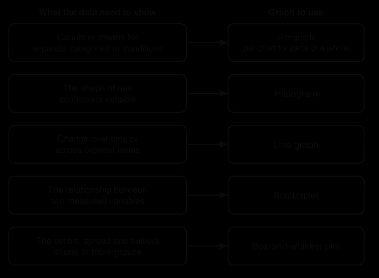
Each common graph answers one kind of question. A study that compares two or more conditions, such as a laptop group and a longhand group, usually reports a mean for each condition, which suits a bar graph. A study of how a behaviour changes with age or over time suits a line graph. A correlational study, which measures two variables in the same participants, needs a scatterplot. When the question is about the shape or spread of one variable, a histogram or a box-and-whisker plot is the right tool.

Frequency tables

The simplest summary of data is a count. A frequency table lists each value or category and the number of times it occurs, often with the percentage of the total. It is the usual first step in organising raw data, and many graphs are simply frequency tables drawn as pictures.

Frequency tables suit nominal data (how many participants showed each attachment type), ordinal data (how many chose each point on a rating scale) and grouped interval or ratio data (how many reaction times fell between 300 and 349 milliseconds, 350 and 399, and so on). With grouped data, the intervals must be equal in width and must not overlap, or the counts cannot be compared.

Hyde (2005) used a frequency table to summarise 124 sex-difference effect sizes from 46 published meta-analyses. An effect size here is the difference between the mean scores of men and women expressed in standard deviation units (the statistic d), so 0.5 means the means are half a standard deviation apart. Grouping the values into size bands turned a long list of studies into five numbers.

Sources: Hyde, J. S. (2005). The gender similarities hypothesis. _American Psychologist, 60(6), 581–592, Table 2._

Reading the table well means checking the total, the base of each percentage and the way categories were formed. The percentages add to 101% because each was rounded, which is normal and worth a footnote. The bands themselves are a choice made by the researcher: had “small” been defined as up to 0.20 rather than 0.35, the table would look different although the data had not changed.

Two-way frequency tables

A two-way table (also called a contingency table or cross-tabulation) counts cases by two categorical variables at once, for example the number of participants in each condition who did and did not report seeing broken glass. Each cell holds one combination. Two-way tables make it possible to compare proportions across groups, but only if the row or column totals are shown, because the same count can be a large or a small share depending on the base.

Bar graphs

A bar graph shows a value for each of several separate categories or conditions as a bar. The bars are separated by gaps, because the categories are distinct, and their order along the horizontal axis can usually be changed without changing the meaning. The height of each bar may show a count, a percentage or, very often in experiments, the mean score of each condition.

Bar graphs are the standard way to report the results of an experiment with a categorical independent variable. Loftus and Palmer’s (1974) speed estimates for five verbs, the conformity rates in different versions of Asch’s procedure, and the mean recall of two groups in a memory study are all bar-graph data. Reading one means stating the value of each bar with its units, comparing the bars (which is highest, which is lowest, how big the gap is), and then asking how much the scores varied inside each bar.

Error bars

A bar for a mean hides every individual score behind it. Two conditions with means of 12 and 14 might contain scores that barely overlap, or scores that overlap almost completely, and the bars alone cannot tell the two apart. Error bars are lines drawn above and below the top of each bar to show the spread or uncertainty around the mean.

Error bars can show different things, so the caption must say which. One standard deviation describes how much individual scores varied. The standard error and the 95% confidence interval describe how precisely the sample mean estimates the population mean, and they shrink as the sample grows. Large error bars that overlap heavily suggest that the difference between two means may be small compared with the variation between people; a graph with no error bars gives no way of judging this.

Pie charts

A pie chart shows the parts of a whole as slices of a circle. It suits a few categories that add up to 100%, such as the percentages of infants classified as secure, avoidant and resistant in a sample. Pie charts are harder to read precisely than bar graphs, because people judge angles and areas less accurately than lengths, so most research reports prefer a bar graph even for proportions. A pie chart can never show means or compare conditions, because the slices must form one whole.

Histograms

A histogram shows how the scores on one continuous variable are spread out. The horizontal axis is divided into equal intervals, and the height of each bar shows how many scores fall into that interval. Because the axis is a continuous scale, the bars touch, and their order cannot be changed. The overall outline of the bars shows the shape of the distribution.

The histogram of national suicide rates shows data for 185 countries in 2021, each country counted once. Most countries fall between 0 and 9 deaths per 100,000 people, with the tallest bar at 6–9 (47 countries). The bars to the right become shorter but continue far out, to a small number of countries above 24. This long right-hand tail is the signature of a positively skewed distribution, and it pulls the mean (8.5) above the median (7.4).

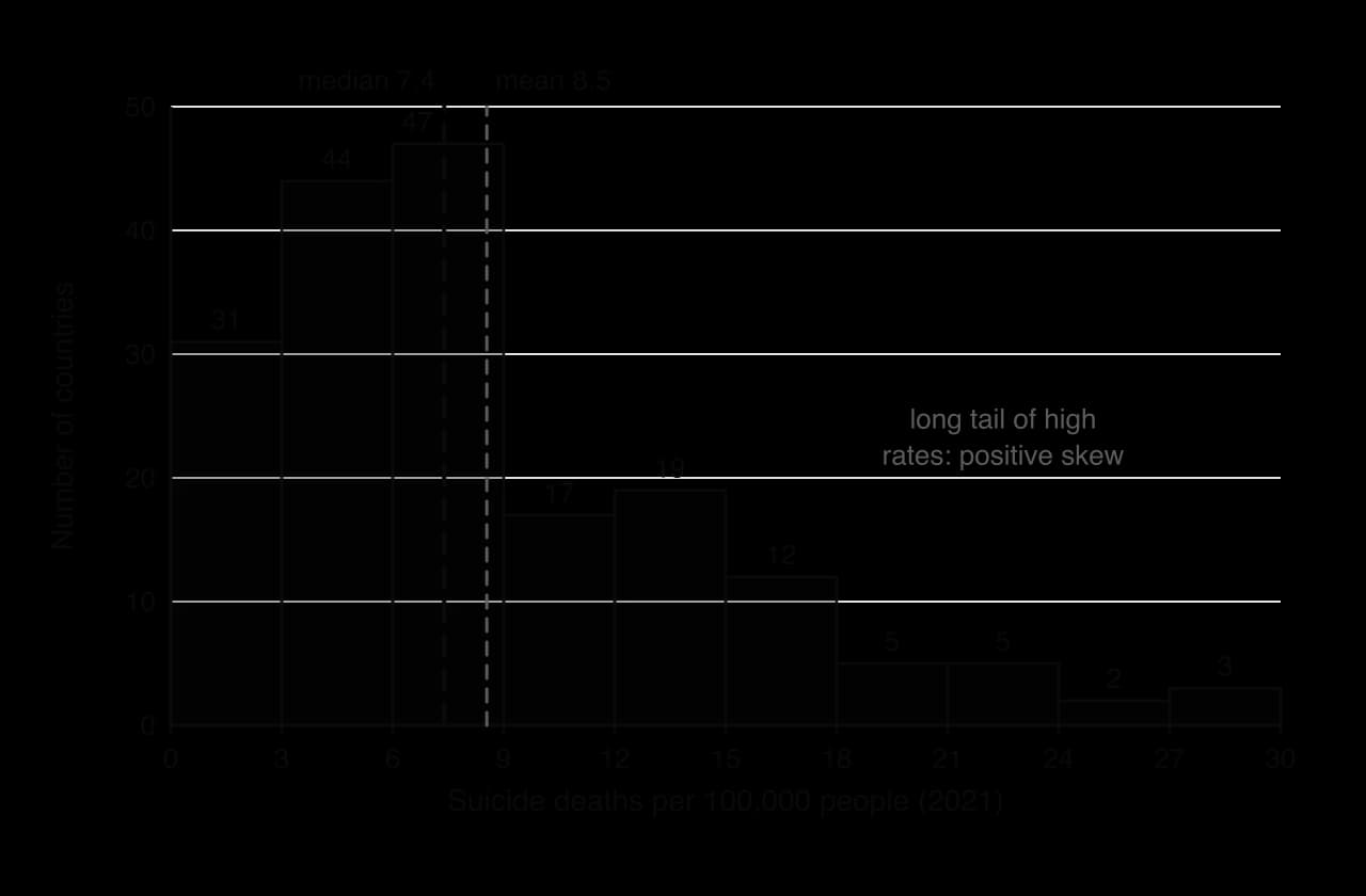
Two choices affect what a histogram appears to show. The first is the width of the intervals (often called bins): very wide bins merge everything into a few bars, and very narrow bins give a jagged picture with many empty intervals. The second is where the first interval starts. A careful reader checks that the intervals are equal and that the vertical axis starts at zero, because a bar’s height is only meaningful when measured from zero.

Real data rarely matches the textbook shapes exactly. Suicide statistics also raise a question of measurement: in countries where suicide is stigmatised or illegal, deaths may be recorded as accidents, so some of the low values on the left of the histogram may reflect under-reporting rather than low rates. A histogram shows the distribution of the recorded numbers, which is not always the distribution of the behaviour itself.

Line graphs

A line graph joins points to show how a variable changes over time or across ordered levels of another variable, such as age groups, sessions of therapy or the number of hours of sleep deprivation. The line suggests that the values between the points follow on from each other, so a line graph is only appropriate when the horizontal axis has a real order. Two or more lines on the same axes allow groups to be compared, for example the progress of a treatment group and a control group across eight weeks.

Reading a line graph means describing the overall trend (rising, falling, stable, rising then falling), the size of the change with numbers from the axis, and any turning points. When two lines are shown, the important question is usually whether the gap between them grows, shrinks or stays the same, because a widening gap may show an interaction between two variables. A line graph of means, like a bar graph, says nothing about the spread around each point unless error bars are included.

The horizontal axis deserves a close look. If the age groups are 7–10, 11–14, 15–18 and 23–59, but the points are spaced equally, the graph makes a 37-year band look the same width as a four-year band, and the slope of the line becomes hard to interpret. A short time window can also mislead: a line that starts in an unusual year may suggest a rise or a fall that disappears when earlier years are added.

Scatterplots

A scatterplot shows the relationship between two variables measured in the same participants (or the same cases, such as countries or schools). Each point represents one participant, placed by their score on one variable along the horizontal axis and their score on the other along the vertical axis. Scatterplots are the standard display for correlational research.

Three features describe the pattern. Direction: in a positive correlation the points rise from left to right (higher scores on one variable go with higher scores on the other); in a negative correlation they fall. Strength: the closer the points lie to a straight line, the stronger the relationship, which the correlation coefficient r summarises on a scale from −1 to +1. Form: the relationship may be linear, or it may curve.

The curvilinear panel shows why a correlation coefficient must always be checked against a scatterplot. Arousal and performance are often described this way (performance rises with arousal up to a point and then falls), and a coefficient near zero would wrongly suggest that the two are unrelated. A line of best fit is often added to a scatterplot to show the direction and slope of a linear relationship.

Anscombe’s quartet: why data must be graphed

The statistician Francis Anscombe (1973) built four small data sets, each of 11 pairs of numbers, to show what summary statistics can hide. All four have the same mean of x (9), the same mean of y (7.50), the same correlation (r = 0.816) and the same line of best fit. Plotted, they look nothing alike.

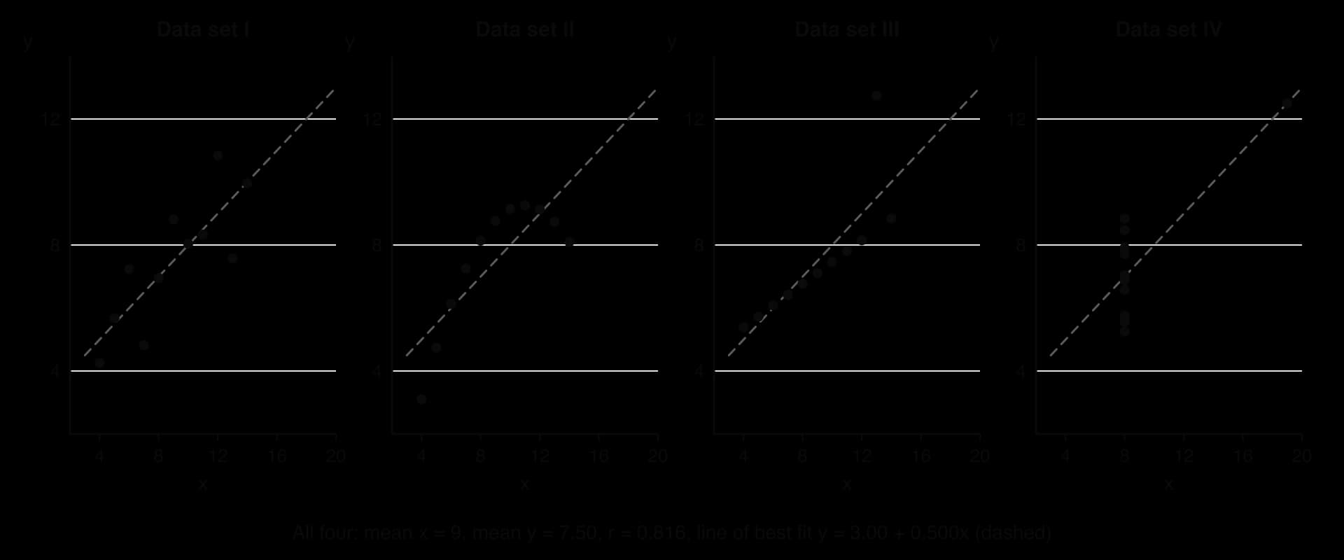
Only data set I matches what r = 0.816 seems to promise. Set II is a smooth curve, so a straight line is the wrong model. In set III, ten points lie almost exactly on a line and one outlier pulls the line of best fit upwards. In set IV, there is no relationship at all among ten of the points, and a single extreme point creates the whole correlation. The same four patterns appear in psychological data, where one unusual participant can create or hide a correlation.

Scatterplots also need careful reading for causality. A positive correlation between hours of social media use and symptoms of depression is compatible with social media causing low mood, with low mood leading to more social media use (bidirectional ambiguity), and with a third variable such as poor sleep or loneliness affecting both. The scatterplot shows only that the scores go together.

Box-and-whisker plots

A box-and-whisker plot (often shortened to box plot) summarises a distribution with five numbers and shows any outliers separately. It is less detailed than a histogram, but several box plots fit side by side on one axis, which makes them the clearest way to compare the centre and spread of several groups at once.

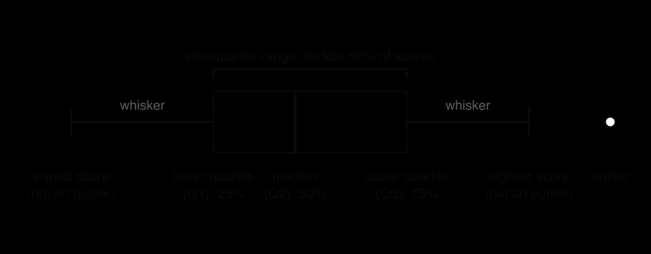
To build one, the scores are put in order and split into four equal parts. The median cuts the data in half. The lower quartile (Q1) is the value below which 25% of the scores fall, and the upper quartile (Q3) the value below which 75% fall. The box runs from Q1 to Q3, so its length is the interquartile range, the spread of the middle half of the data. The whiskers extend to the lowest and highest scores that are not outliers; a common rule treats any score more than 1.5 interquartile ranges below Q1 or above Q3 as an outlier and marks it as a separate point.

A box plot shows skew as well as spread. In a symmetrical distribution, the median sits in the middle of the box and the two whiskers are about the same length. When the median is close to one end of the box and the whisker on the other side is long, the distribution is skewed towards the long whisker.

Comparing groups with box plots

The regional box plots use the same national suicide rates as the histogram, split into five World Bank regions. Each box summarises the countries of one region, so the figure compares five distributions at once. South Asia (6 countries) and North America (2) are left out because a box plot of so few values would be misleading.

Several patterns can be read directly. The median rate is lowest in the Middle East, North Africa, Afghanistan and Pakistan region (about 2.9 per 100,000) and highest in Europe and Central Asia (about 11.5). Spread varies more than the medians: the box for East Asia and Pacific runs from about 4.5 to 16.4, an interquartile range of nearly 12, while the box for Sub-Saharan Africa runs only from about 5.3 to 8.6. Sub-Saharan Africa also has five high outliers, including Lesotho (28.7) and Eswatini (27.2), so the region’s mean would be a poor summary of a typical country.

The box plots also show the limits of grouped data. Each point is a country, not a person, so a high regional median says nothing about the risk of any individual living there; drawing that inference would be an ecological fallacy. The regions differ in how deaths are recorded, in how many countries they contain (from 23 to 48 here) and in culture, religion and access to means, so the graph raises questions rather than answering them.

Distributions and their shapes

A distribution is the pattern formed by all the scores in a data set: which values occur and how often. Histograms, box plots and smooth curves are all ways of picturing it. Three features describe any distribution: its shape (symmetrical or skewed, one peak or two), its centre (described by the mean, median or mode) and its spread (described by a measure of dispersion such as the range or the standard deviation).

The normal distribution

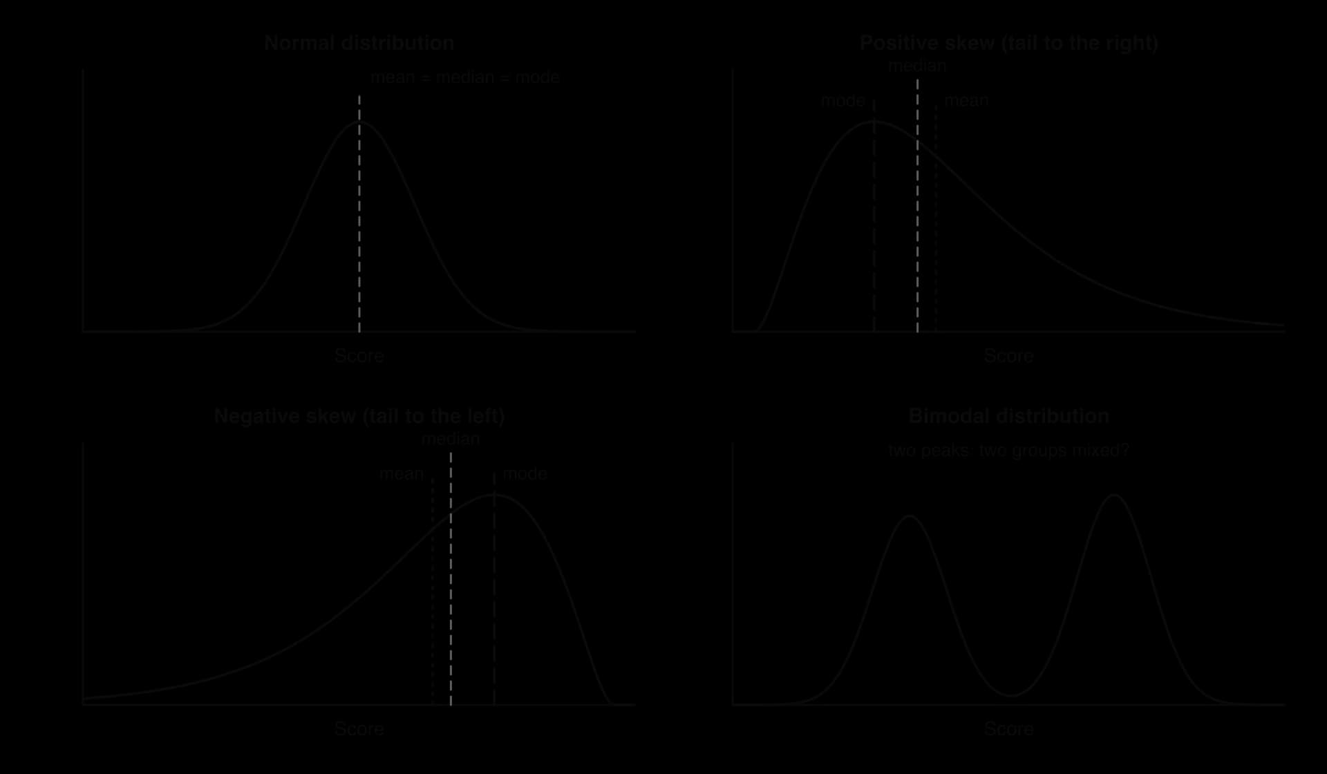
Many psychological variables, especially those that result from many small independent influences, form a normal distribution: a symmetrical, bell-shaped curve with most scores close to the centre and fewer and fewer towards each end. Height, scores on well-designed ability tests and many measures of personality are roughly normal. In a perfectly normal distribution, the mean, median and mode are the same value.

The normal curve has a fixed relationship with the standard deviation. About 68% of scores lie within one standard deviation either side of the mean, about 95% within two, and about 99.7% within three. Intelligence tests, for example, are standardised so that scores have a mean of 100 and a standard deviation of 15, which places about two-thirds of people between 85 and 115. Many inferential statistics assume that the data are roughly normal, so checking the shape of a distribution is the first step before choosing how to analyse it.

Skewed distributions

A distribution is skewed when one tail is longer than the other. Skewness is named after the direction of the tail, not the peak. In a positive skew (skewed to the right), most scores are low and a few are very high: reaction times, the number of days in hospital and income all take this shape. In a negative skew (skewed to the left), most scores are high and a few are very low: scores on an easy test and age at death in high-income countries are examples.

Skew often comes from a limit on one side of the scale. Time cannot be less than zero, so reaction times bunch up near the fastest possible response and stretch out to the right. Tests show the same pattern. A test that is too difficult produces a floor effect, with many participants scoring at or near the minimum and a tail of higher scores (positive skew). A test that is too easy produces a ceiling effect: many participants score at or near the maximum, and only a few score low (negative skew). Floor and ceiling effects are a problem of measurement as well as of shape, because a test that most people pass cannot tell apart the people who passed it easily from those who only just passed.

Skew moves the three averages apart in a predictable order. The mode stays at the peak, the median is the middle score, and the mean is pulled furthest towards the long tail because it uses the actual values of the extreme scores. So in a positive skew the order from left to right is mode, median, mean, and in a negative skew it is mean, median, mode. The national suicide data follow this pattern: the modal interval is 6–9, the median 7.4 and the mean 8.5.

Bimodal distributions

A bimodal distribution has two clear peaks. It often shows that two different groups have been mixed in one data set, such as children and adults in a sample measured on vocabulary, or participants who understood a task and participants who did not. Reporting a single mean for a bimodal distribution describes almost nobody: the mean may fall in the dip between the peaks, where very few scores lie. The right response is usually to look for the variable that separates the two groups and analyse them separately.

YouTube

Outliers

An outlier is a score that lies far from the others. It may be a genuine but unusual case (a participant with an exceptional memory), the result of an error (a reaction time of 9,000 milliseconds because the participant was distracted, or a data-entry mistake that turned 19 into 91), or a sign that a participant did not follow the instructions. Outliers matter because some statistics are very sensitive to them.

The mean uses the value of every score, so one extreme value can move it a long way. In the scores 4, 5, 5, 6, 6, 7 and 42, the median is 6, but the mean is 75 ÷ 7 ≈ 10.7, higher than six of the seven scores. The median and the interquartile range depend only on the order of the scores, so they barely change. This is why the median and interquartile range are preferred for data with outliers or strong skew.

What researchers do with outliers

There is no single correct way to handle an outlier, but there is a correct order of thinking. First, the researcher checks whether the value is an error; if it is, it is corrected or removed. Second, if it is a real score, the researcher decides whether it belongs to the population being studied (a participant who misunderstood the task may be excluded, with the reason reported). Third, the analysis can be run with and without the outlier to see whether the conclusion depends on it.

The rule for excluding outliers should be decided before the data are collected and reported in full. If researchers look at their results first and then remove whichever extreme scores weaken their hypothesis, the exclusion becomes a form of p-hacking and introduces researcher bias into the findings. Pre-registration, in which the analysis plan is published before data collection, is one safeguard.

What limits the interpretation of a table or graph

A graph is accurate only when it is drawn and read accurately, and even an honest graph shows only part of the picture. Interpreting data means asking, for each table or graph, what it shows, how it was produced and what it cannot show. The same problems come up again and again in published research, news reports and summaries of studies.

Truncated axes

A truncated axis starts at a value other than zero. On a bar graph this changes the ratio between the bars’ heights, so small differences look large. The same five means from Loftus and Palmer (1974) can be drawn twice: once with the vertical axis from zero and once from 30 miles per hour.

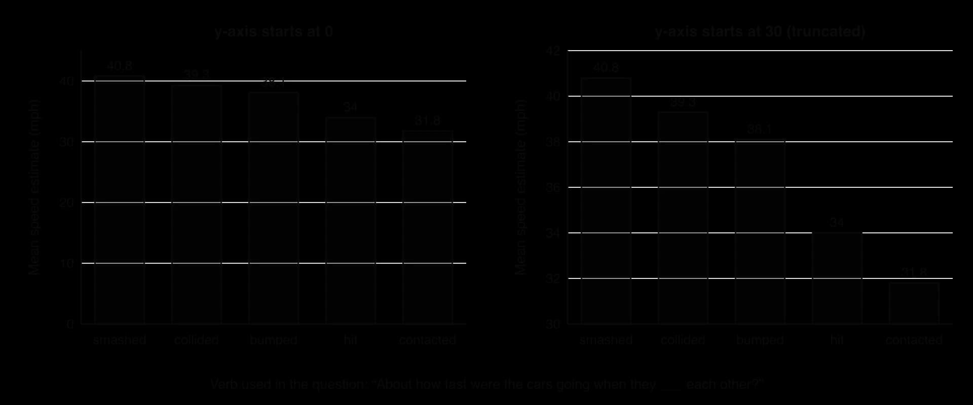
A truncated axis is not always dishonest. Line graphs of variables that never come near zero, such as body temperature, are easier to read with a narrow axis, and a break symbol on the axis tells the reader that part of the scale is missing. On bar graphs, where the reader compares lengths, an axis that does not start at zero almost always exaggerates.

YouTube

A checklist of common issues

Evaluating data displays through the concepts

Tables and graphs are part of the research process, so they can be evaluated through the same concepts as any study. The table links the most common issues to the concepts they raise.

Key study: Hyde (2005), the gender similarities hypothesis

Aim

Janet Shibley Hyde aimed to test the gender similarities hypothesis: the idea that males and females are similar on most, but not all, psychological variables. She contrasted it with the “differences model” common in popular books and the media, which presents men and women as psychologically very different. The question was one of distributions: how far apart are the scores of males and females on psychological measures, and how much do their distributions overlap?

Method

Hyde reviewed 46 published meta-analyses of psychological gender differences. Each meta-analysis had already combined the results of many studies of one variable. Together they covered six areas: cognitive variables (such as mathematics, verbal and spatial abilities), verbal and nonverbal communication (such as interruptions and smiling), social and personality variables (such as aggression, helping and leadership), psychological well-being (such as self-esteem), motor behaviours (such as throwing distance) and miscellaneous constructs (such as moral reasoning). Where possible, she used recent meta-analyses with large samples, including some large national probability samples of adolescents.

The size of each difference was measured as d, the difference between the male mean and the female mean divided by the average standard deviation within each sex. A positive d meant that males scored higher, and a negative d that females scored higher. Of 128 effect sizes, four could not be classified because the meta-analysis gave too wide a range. The remaining 124 were sorted into five size bands based on the conventions of the statistician Jacob Cohen: close to zero (d ≤ 0.10), small (0.11–0.35), moderate (0.36–0.65), large (0.66–1.00) and very large (over 1.00).

Results

Of the 124 effect sizes, 37 (30%) were close to zero and 59 (48%) were small, so 78% of the gender differences were small or close to zero. Nineteen (15%) were moderate, seven (6%) large and two (2%) very large. The distribution of effect sizes is itself positively skewed: most values cluster near zero, with a short tail of large differences.

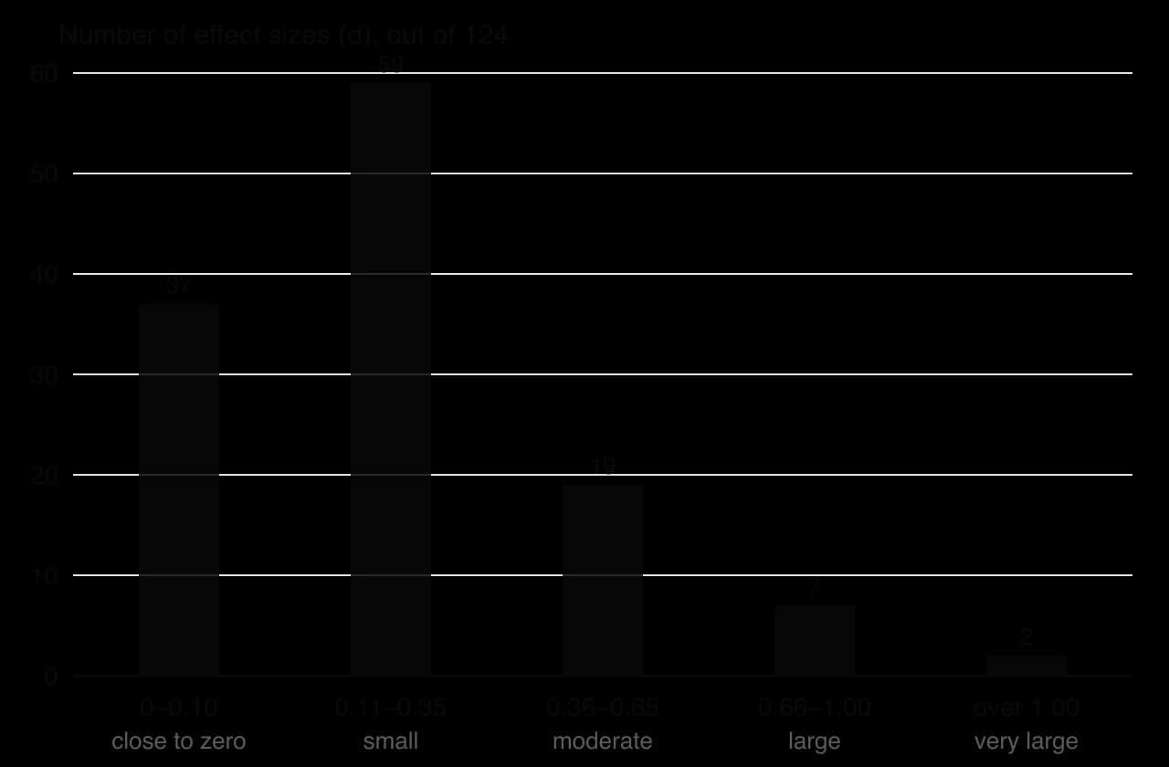
Variables close to zero included mathematics problem solving (d = 0.08), reading comprehension (d = −0.09 in national samples) and leadership effectiveness (d = −0.02). The largest differences were in motor performance after puberty, such as throwing velocity (d = 2.18) and throwing distance (d = 1.98), some measures of sexuality, such as attitudes about casual sex (d = 0.81), and physical aggression, which was moderate (d = 0.60 in one meta-analysis). Spatial ability depended on the task: mental rotation showed a moderate-to-large difference (d = 0.56 and 0.73 in two meta-analyses), while spatial visualisation was small (d = 0.13 and 0.19).

To show what a small effect means for individuals, Hyde reproduced a graph of two normal distributions 0.21 standard deviations apart, the approximate gender difference in self-esteem found by Kling et al. (1999). The same idea can be drawn for any value of d.

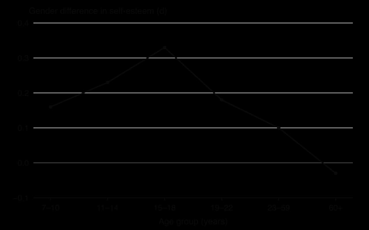
Two further findings concerned age and context. Differences rose and fell across the lifespan: for self-esteem, d was 0.16 at ages 7–10, 0.33 at 15–18 and 0.10 at 23–59, and slightly favoured women over 60 (d = −0.03). Context changed the size of differences too. Women smiled more than men overall (d = −0.40), but the difference was larger when people knew they were being watched (d = −0.46) than when they did not (d = −0.19).

Conclusions

Hyde concluded that the data supported the gender similarities hypothesis: on most psychological variables, the distributions of males and females overlap heavily, so knowing a person’s sex says very little about their score. The few large differences are real and should be recognised. Because the size of a difference changes with age and with the social context of measurement, gender differences cannot be treated as large, fixed traits. Hyde argued that overstated claims of difference have costs, for example in hiring, in education and in how couples interpret conflict.

Evaluation

Measurement: what a single number hides

The study is a strong demonstration that a difference between two means must be read alongside the distributions behind it. However, the classification depends on choices about measurement. The size bands are conventions rather than natural categories; moving the boundary of “small” would change the bar graph. Effect sizes also depend on how a construct is measured: in one meta-analysis Hyde cites, relational aggression showed a moderate difference favouring girls when observed directly (d = −0.45) but almost none in self-reports (d = −0.02).

A further critique concerns combining variables. Del Giudice, Booth and Irwing (2012) measured 15 personality factors in a representative US sample of 10,261 adults and combined them into one multivariate effect size. Although most single factors showed small or moderate differences, the overall profiles of men and women overlapped by only about 10%. Whether gender differences look “small” therefore depends partly on whether variables are analysed one at a time or together.

Bias: which samples and which studies

Most of the meta-analyses drew on studies from the United States and other Western, often student, samples, so the review says little about cultures with very different gender roles. This matters because the context findings suggest that the size of differences depends on social roles and expectations. Publication bias is also possible: studies that find a significant difference may be more likely to be published than studies that find none, which, if anything, would make the published differences look larger than they are and strengthen Hyde’s conclusion.

Responsibility: communicating group differences

Research on group differences is socially sensitive, because popular reports often turn averages into claims about every man or every woman. By presenting effect sizes and overlapping distributions rather than only “significant differences”, Hyde showed a responsible way to communicate such findings. The same reasoning applies to any comparison of groups, such as cultures, age groups or patients and controls.

Sources: Hyde, J. S. (2005). The gender similarities hypothesis. _American Psychologist, 60(6), 581–592. Del Giudice, M., Booth, T., & Irwing, P. (2012). The distance between Mars and Venus: Measuring global sex differences in personality. PLoS ONE, 7(1), e29265._

Exam practice

Graphs and tables are the raw material of Paper 3. Its sources are built around a claim about culture, motivation or technology in one context, and the first two questions test graph- and table-reading skills directly: explaining an issue that limits the interpretation of a source (3 marks), and analysing a source’s findings and stating a conclusion linked to the claim (6 marks). The qualitative question (6 marks) and the synthesis essay (15 marks) draw on every source, including the graphs. The practice set uses one invented resource booklet throughout.

Practice resource booklet (hypothetical data). The sources have been collated to assess the claim that using a smartphone in bed harms adolescents’ sleep.

• Source 1. A bar graph from a school newsletter shows mean sleep per night for students who “keep their phone in the bedroom” (7.1 hours) and those who “do not” (7.4 hours). The vertical axis runs from 7.0 to 7.5 hours. No sample size or error bars are given.

• Source 2. A survey of 600 students aged 13–17 in one country. Screen time after 10 p.m. (self-reported, hours) correlated with time taken to fall asleep (self-reported, minutes): r = 0.21. Mean time to fall asleep was 18 minutes (SD 9) for students with no screen use after 10 p.m., 24 minutes (SD 13) for up to one hour, and 31 minutes (SD 21) for more than one hour. The distribution of time to fall asleep was positively skewed.

• Source 3. Focus groups with 18 students aged 15–16 at one boarding school, run by the school counsellor. Thematic analysis produced three themes: “fear of missing out at night”, “the phone as a way to fall asleep” and “rules that nobody follows”.

• Source 4. A two-week field experiment: 80 students were randomly allocated to hand in their phones at 9 p.m. or to keep them. Box plots of sleep duration (measured with wrist-worn devices) show a median of 7.6 hours (IQR 7.1–8.0) for the phone-free group and 7.2 hours (IQR 6.5–7.9) for the control group, with two control-group outliers below 5 hours.

The analysis question asks for more than a description: the numbers must be compared, the design and measures weighed, and the conclusion tied to the claim with appropriate caution.

The synthesis question rewards using at least three sources, weighing their strengths against each other and adding knowledge from beyond the booklet. A source’s graph type and design decide how much weight it can carry.

Summary

• The study design (comparison, change over time, relationship) and the level of measurement (nominal, ordinal, interval, ratio) decide which table or graph is appropriate.

• Frequency tables count cases per category or interval; percentages must always be read against their base numbers.

• Bar graphs compare separate categories or conditions (gaps between bars); histograms show the distribution of one continuous variable (touching bars); line graphs show change across ordered levels or time.

• Scatterplots show the direction, strength and form of a relationship; Anscombe’s quartet shows that identical statistics can hide very different patterns, and correlation never shows causation.

• Box-and-whisker plots show the median, quartiles, interquartile range and outliers, and are best for comparing the spread of several groups.

• In a normal distribution the mean, median and mode are equal; in a positive skew the tail is on the right and the mean is highest; in a negative skew the tail is on the left and the mean is lowest; a bimodal shape suggests two groups.

• Outliers distort the mean and correlations far more than the median; rules for excluding them should be set in advance and reported.

• Interpretation is limited by truncated axes, missing spread or sample size, measures that do not match the claim, correlational designs and aggregated data.

• Hyde (2005) found that 78% of 124 gender-difference effect sizes were small or close to zero, showing that a difference between means can hide heavily overlapping distributions.

Self-check

• To do:

  I can explain how the design of a study and its level of measurement decide how data is represented.

• To do:

  I can describe what each kind of table and graph shows and choose the right one for a study.

• To do:

  I can interpret a frequency table, bar graph, histogram, line graph, scatterplot and box plot using its numbers.

• To do:

  I can describe normal, skewed and bimodal distributions and place the mean, median and mode in each.

• To do:

  I can explain how outliers arise, how they affect the mean and how researchers should deal with them.

• To do:

  I can explain at least five issues that limit the interpretation of a table or graph.

• To do:

  I can describe and evaluate Hyde (2005) as an example of interpreting distributions and effect sizes.

• To do:

  I can evaluate data displays with reference to measurement, bias and causality.