Notes on 2.1 Individuals, populations, communities, and ecosystems
Learning objectives
Outline the levels of ecological organisation from the individual to the biosphere, and define species, population, community, habitat and ecosystem.
Explain how binomial nomenclature and classification help identification, and use a dichotomous key.
Describe how abiotic factors are measured and how abiotic and biotic factors affect the distribution of a species.
Outline the niche of a named species and describe examples of herbivory, predation, parasitism, mutualism, disease and competition.
Explain carrying capacity, density-dependent regulation by negative feedback, and J-, S- and boom-and-bust growth curves.
Discuss why the carrying capacity of the human population is difficult to assess.
Evaluate random, systematic and transect sampling, and calculate percentage cover, percentage frequency, density and the Lincoln index.
Explain why ecosystems are open systems that can be sustainable, and how human activity can push them past a tipping point.
Explain the role of keystone species and why biosphere integrity is a crossed planetary boundary.
Interpret cladograms and outline the difficulties of the traditional hierarchy of taxa. (HL)
Distinguish fundamental and realised niches, and r- and K-strategists, using named examples. (HL)
Explain how knowledge of classification, niches and life cycles helps predict human impacts such as phenological mismatch. (HL)
Introduction
Ecology is the study of how living things interact with each other and with their physical surroundings. It explains why a species lives where it does, why its numbers rise and fall, and why some ecosystems last for millions of years while others collapse within a few decades.
These questions matter well beyond biology. Fisheries, farming, forestry and conservation all depend on predicting how populations respond to change, and the same ideas of limits and feedback apply to the human population. The systems approach is used throughout ecology: an ecosystem is treated as a system with storages, flows and feedback loops, and its sustainability depends on whether its inputs and outputs stay in balance. Different perspectives then shape what societies decide to do about the changes that ecologists measure.
Levels of ecological organisation
Ecologists study life at several levels, each built from the one below it. A single organism belongs to a population of its species; populations of different species living together form a community; a community and its physical surroundings form an ecosystem; and all the ecosystems on Earth together make up the biosphere.
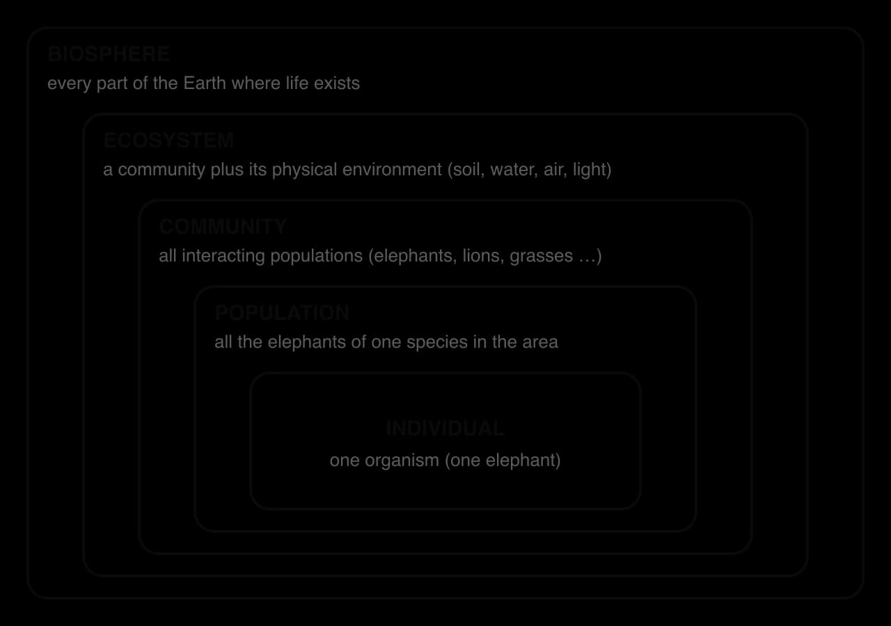
The biosphere is thin compared with the size of the planet. Most life is found within a few kilometres of the surface: from the deep ocean floor to a few kilometres up in the atmosphere. Within it, matter is recycled and energy flows through every level, which is why the biosphere is studied as one large system made of many smaller ones.
Each level has properties that the level below it does not. A population has a birth rate and a density, which a single organism cannot have; a community has a food web; an ecosystem cycles nutrients. These are examples of emergent properties, which appear only when the parts interact.
Individuals and species
An individual organism is always a member of a species. For animals and many plants, the most widely used way to decide where one species ends and another begins is the biological species concept: members of a species can breed with each other and produce fertile offspring, but not with members of other species.
A horse and a donkey can mate, but their offspring, the mule, is almost always sterile, so horses and donkeys are separate species. Lions and tigers can produce hybrids in captivity, but in the wild they live in different places and do not interbreed, so they are kept as separate species too.
Where the biological species concept struggles
The definition depends on breeding, so it cannot be applied directly to organisms that reproduce without sex, such as many bacteria and some plants, or to extinct species known only from fossils. Some closely related species also hybridise occasionally in the wild. In these cases biologists decide species boundaries using shared physical features or DNA sequences instead. The definition is a model: useful for most animals, but a simplification of a messy reality.
Populations
A population is the unit in which a species actually lives and breeds. All the members of a species are rarely in one place: the African savanna elephant, for example, lives in many separate populations across eastern and southern Africa, each in a different area. A species can therefore consist of a single population, if its range is small, or of hundreds of populations.
Populations are the level at which numbers change. Births and immigration add individuals; deaths and emigration remove them. Most of the ideas about growth, carrying capacity and regulation that follow are ideas about populations.
Communities and habitats
Populations do not live alone. On a rocky shore, barnacles, mussels, limpets, seaweeds and sea stars live together, eat one another, compete for space and shelter each other. The populations of all the species living and interacting in one area form a community.
The place where an organism, population or community lives is its habitat. A description of a habitat gives its location and the physical conditions found there. The habitat of the common frog, for example, includes ponds for breeding and damp grassland and woodland nearby for feeding, within a temperate climate.
Classifying and identifying organisms
Well over a million species of animals, plants, fungi and microorganisms have been described by scientists, and many more remain unknown. Without a system for naming and grouping them, nobody could be sure which organism another person was describing. Classification solves this by sorting organisms into groups by their shared features.
A good classification does more than name things. Species in the same group share many features, so knowing the group of a newly found organism allows predictions about it: a newly discovered beetle can be expected to have six legs, hard wing cases and a life cycle with a larva and a pupa, before anyone has studied it.
Binomial nomenclature
Every species has a two-part scientific name, an idea introduced by the Swedish botanist Carl Linnaeus in the 18th century. This system is called binomial nomenclature. The first part is the genus and starts with a capital letter; the second part identifies the species and is all in lower case. The name is printed in italics, or underlined when handwritten.
Common name | Scientific name | Genus | Species name |
|---|---|---|---|
Human | Homo sapiens | Homo | sapiens |
Purple sea star (ochre sea star) | Pisaster ochraceus | Pisaster | ochraceus |
Koala | Phascolarctos cinereus | Phascolarctos | cinereus |
Reindeer (caribou) | Rangifer tarandus | Rangifer | tarandus |
Lion | Panthera leo | Panthera | leo |
Tiger | Panthera tigris | Panthera | tigris |
The same scientific name is used in every language, which avoids confusion between common names. “Robin” refers to a small red-breasted bird (Erithacus rubecula) in Britain but to a much larger thrush (Turdus migratorius) in North America. Lions and tigers share the genus Panthera, which tells a reader that they are closely related big cats.
Tools for identifying organisms
Taxonomy is the science of naming, describing and classifying organisms, and taxonomists use several tools to work out which species an unknown specimen belongs to. In fieldwork the most common is a dichotomous key, but comparison with reference collections and analysis of DNA are often used alongside it.
Dichotomous keys
A dichotomous key is a series of numbered questions, each with two possible answers. Each answer leads either to another question or to the name of an organism. The user works through the key from the first question, choosing the description that fits the specimen, until a name is reached. Good keys use features that are easy to see and do not change with age, season or sex, such as the number of legs, rather than colour or size.

Reference collections, DNA and digital tools
A reference collection is a set of correctly identified specimens kept in a museum, herbarium or university. An unknown specimen can be compared directly with them. Large collections such as those of natural history museums hold millions of specimens, including the “type specimen” on which the original description of each species was based.
DNA barcoding identifies a species from a short, standard section of its DNA. In animals this is usually part of a mitochondrial gene called cytochrome c oxidase I (COI); in plants, sections of two chloroplast genes are used. The sequence is compared with a reference library such as the Barcode of Life Data System. Barcoding can identify eggs, larvae, fragments or processed food that have no useful visible features, and it can show that what looked like one species is really several. In north-western Costa Rica, barcoding suggested that the butterfly Astraptes fulgerator was a group of about ten very similar species, although later work argued for fewer.
Environmental DNA (eDNA) takes the idea further: traces of DNA shed into water or soil are sequenced to detect which species are present in a lake or a field without ever catching them. Smartphone apps and online databases such as iNaturalist compare photographs with millions of identified records, which lets volunteers in citizen science projects record species, although expert checking is still needed for difficult groups.
Tool | Strengths | Limitations |
|---|---|---|
Dichotomous key | Cheap and quick in the field; teaches observation of features | Only covers the species it was written for; needs a whole, adult specimen; users may misread features |
Reference collection | Direct comparison with expertly identified specimens | Kept in museums, so the specimen must be collected and taken there; needs expert staff |
DNA barcoding and eDNA | Works on fragments, larvae and look-alike species; can detect rare or hidden species | Needs a laboratory and a complete reference library; costly; contamination risk |
Apps and databases | Instant; many users; records add to large datasets | Accuracy varies with photo quality and with how well a group is covered; needs expert checking |
What controls where a species lives
No species lives everywhere. Mangrove trees grow along tropical coasts but not in the Sahara; brown trout live in cool, fast, well-oxygenated streams but not in warm, stagnant ponds. The distribution of a population, meaning where it is found, depends on the conditions around it. Ecologists divide these conditions into two kinds: biotic factors, which come from living things, and abiotic factors, which do not.
Abiotic factors are the non-living, physical and chemical conditions. Temperature, sunlight, pH, salinity, dissolved oxygen and soil texture are among the most important. Wind speed, water flow, soil moisture, altitude and slope matter in particular places.
Each species can survive only within a certain range of each abiotic factor, its range of tolerance. Near the middle of the range individuals grow and reproduce well; towards either end they become stressed, and beyond it they die. Brown trout, for example, need cool water with plenty of dissolved oxygen, because warm water holds less oxygen. A species is usually found where all the factors that matter to it fall inside its ranges of tolerance at the same time, and where biotic factors such as competitors and predators allow it to persist.
Abiotic factor | Why it affects distribution | Example |
|---|---|---|
Temperature | Controls the rate of metabolism and enzyme activity; extremes kill | Coral reefs grow only in warm, shallow tropical seas |
Sunlight (light intensity) | Energy for photosynthesis; plants and algae need enough light | Seaweeds and seagrasses grow only in shallow, well-lit water |
pH | Affects nutrient availability in soil and the survival of aquatic animals | Many snails and crayfish are absent from very acidic streams |
Salinity | Salt draws water out of cells that are not adapted to it | Mangroves and salt-marsh plants tolerate salty water; most crops do not |
Dissolved oxygen | Aquatic animals need it for respiration | Mayfly nymphs and trout disappear from low-oxygen water |
Soil texture | The mix of sand, silt and clay controls drainage, water holding and air in the soil | Heather grows on free-draining sandy soils; rushes on waterlogged clay |
Measuring abiotic factors
Abiotic factors can be measured, which turns a description such as “shady and wet” into numbers that can be compared between sites and linked to the distribution of species. Many are measured with electronic probes connected to a data logger, which records readings automatically at set intervals, for example every ten minutes for a week.
Factor | Method | Limitations to evaluate |
|---|---|---|
Temperature (air, water or soil) | Thermometer or temperature probe; data logger for changes over time | Varies through the day, so single readings must be taken at the same time; sun on the probe gives false highs |
Light intensity | Light meter (lux meter) held at the same height and angle | Changes with every passing cloud; take several readings and use the mean |
pH | pH meter or probe; universal indicator paper for a rough value | Probes need calibrating with buffer solutions; indicator colours are judged by eye |
Salinity | Conductivity meter, refractometer or salinity probe | Readings change with temperature; meters need calibrating |
Dissolved oxygen | Oxygen probe (or a chemical titration) | Changes quickly with temperature, photosynthesis and turbulence; measure on site |
Soil texture | Sieving a dried sample, a sedimentation test in a jar, or the ribbon test by hand | The hand test is subjective; sieving and sedimentation take time |
Water flow velocity | Flow meter, or timing a float over a measured distance | Floats move with surface current only and are blown by wind |
Wind speed | Anemometer | Gusty; needs repeated readings at a fixed height |
The niche
Where a species lives is only part of the story. To understand why it survives there, ecologists describe everything it depends on and everything it does: its food, the conditions it tolerates, when it is active, how it avoids predators and where it breeds. Together these make up its niche.
The koala (Phascolarctos cinereus) of eastern and southern Australia shows how narrow a niche can be. Its habitat is open eucalyptus woodland, and its niche can be described by several parameters.
Niche parameter | The koala |
|---|---|
Food | Leaves of eucalyptus trees, a diet low in nutrients and containing toxic compounds; it prefers about 30 of the more than 600 eucalyptus species and eats up to about 400 g of leaves a day |
Water | Gets most of its water from leaves and rarely drinks |
Energy budget | A low-energy lifestyle: a metabolic rate about half that of a typical mammal, and around 20 hours a day asleep or resting |
Adaptations to the diet | A very large caecum in which microorganisms help to break down tough leaves |
Activity and shelter | Mostly active at night, living in the trees |
Predators | Few: occasionally dingoes, large pythons and some birds of prey |
A niche this specialised makes the koala vulnerable. If its preferred eucalyptus species are cleared for farmland or housing, or burned in bushfires, it has few alternatives, which is one reason the IUCN lists it as Vulnerable and it was listed as Endangered in Queensland, New South Wales and the Australian Capital Territory in 2022.
Sources: Wikipedia, “Koala” (read 2026), citing the Australian Government and IUCN.
How populations interact
Populations in a community affect each other in six main ways. In some interactions both species gain, in others one gains at the other’s expense, and in competition both lose something. These interactions drive population dynamics, changing the size of populations, the way individuals behave and, over many generations, the features of the species themselves.
Interaction | What happens | Effect (+ gains, − loses) | Example |
|---|---|---|---|
Herbivory | An animal eats plants or algae | Herbivore +, plant − | African savanna elephants strip bark and push over acacia trees |
Predation | A predator kills and eats its prey | Predator +, prey − | Canada lynx (Lynx canadensis) hunting snowshoe hares |
Parasitism | A parasite lives on or in a host, feeding from it, usually without killing it quickly | Parasite +, host − | The mite Varroa destructor feeding on honeybees |
Mutualism | Two species live closely together and both benefit | Both + | Mycorrhizal fungi on plant roots: the fungus supplies water and minerals, the plant supplies sugars |
Disease | A pathogen (a virus, bacterium, fungus or protist) infects a host and harms it | Pathogen +, host − | The chytrid fungus Batrachochytrium dendrobatidis killing frogs |
Competition | Two or more organisms need the same limited resource | Both − | Red and grey squirrels competing for seeds in British woodland |
Competition within and between species
Intraspecific competition takes place between members of the same species. Reindeer on an island all eat the same lichens, and as their numbers rise each animal gets less. Intraspecific competition is especially strong because individuals of the same species have exactly the same needs.
Interspecific competition takes place between different species. The North American grey squirrel (Sciurus carolinensis) was introduced to Britain in the 1870s. It digests acorns more efficiently than the native red squirrel (Sciurus vulgaris), raids red squirrels’ food stores and lives at higher densities in broadleaved woods, so it takes a larger share of the food. Red squirrels have disappeared from most of England and survive mainly in Scotland and on islands such as Anglesey and the Isle of Wight.
Disease as an interaction
Disease can reshape whole communities. Chytridiomycosis, caused by a fungus spread around the world by human trade, has contributed to the decline of at least 501 amphibian species over the past half-century, including about 90 presumed extinctions, mostly in the wet tropics of the Americas and in Australia. It is the greatest recorded loss of biodiversity attributed to a single disease.
Sources: Scheele et al., _Science (2019)._
Predator–prey relationships
The populations of a predator and its prey often rise and fall in linked cycles. When prey are plentiful, predators eat well, survive and breed, so their numbers rise. More predators then kill more prey, and the prey population falls. With less food, predators starve or fail to breed, so their numbers fall too. With fewer predators, the prey recover, and the cycle begins again.
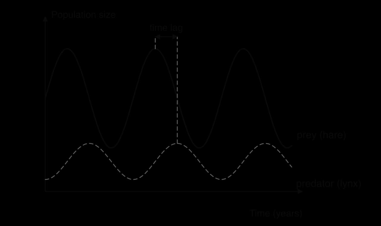
The best-known example is the snowshoe hare and the Canada lynx in the boreal forests of Canada. Fur-trading records kept by the Hudson’s Bay Company since the 1730s show hare scarcity returning every eight to eleven years, with lynx numbers following. Snowshoe hares make up about 35–97% of the lynx diet, depending on the season and on how many hares there are. The real cycle is more complicated than the simple model: hare numbers also depend on the amount of winter food, so the predator is not the only cause.
Interactions have consequences at three levels. Ecologically, they change population sizes and can keep a population near its carrying capacity. Behaviourally, prey change what they do: hares stay closer to cover when lynx are common, and grazing animals form herds. Evolutionarily, interactions act as selective pressures: predators that are slower or less skilful leave fewer offspring, and so do prey that are easier to catch, so both populations change over many generations.
 YouTube
Carrying capacity and limiting factors
No population can grow for ever, because the resources it needs are limited. Food, water, space, light, nesting sites and shelter are all in finite supply. Once a population is large enough to use most of them, individuals compete for what is left, and the population stops growing. The size at which this happens is the carrying capacity of the environment for that species.
The resource that runs short first sets the limit, and is called a limiting factor. Limiting factors can be abiotic, such as water in a desert, light for plants on a forest floor or nest holes in old trees for some birds, or biotic, such as the supply of prey for a predator or of flowers for a pollinator.
Carrying capacity is not a fixed number. A wet year raises the carrying capacity of a grassland for grazing animals and a drought lowers it. A population that damages its own resources, for example by overgrazing slow-growing plants, can also lower the carrying capacity for the future.
Density-dependent and density-independent factors
Some factors that affect birth and death rates become stronger as a population becomes more crowded. These density-dependent factors include competition for food and space, predation (predators find prey more easily and may switch to the most common prey) and disease (pathogens and parasites spread more easily between individuals that live close together). Stress from crowding can also reduce breeding in some mammals.
Other factors kill a similar proportion of the population whatever its density. These density-independent factors are usually abiotic: a severe winter, a drought, a flood, a fire or a volcanic eruption. They can cause sudden, large changes in numbers, but they do not regulate a population, because their effect does not depend on how crowded it is.
Regulation by negative feedback
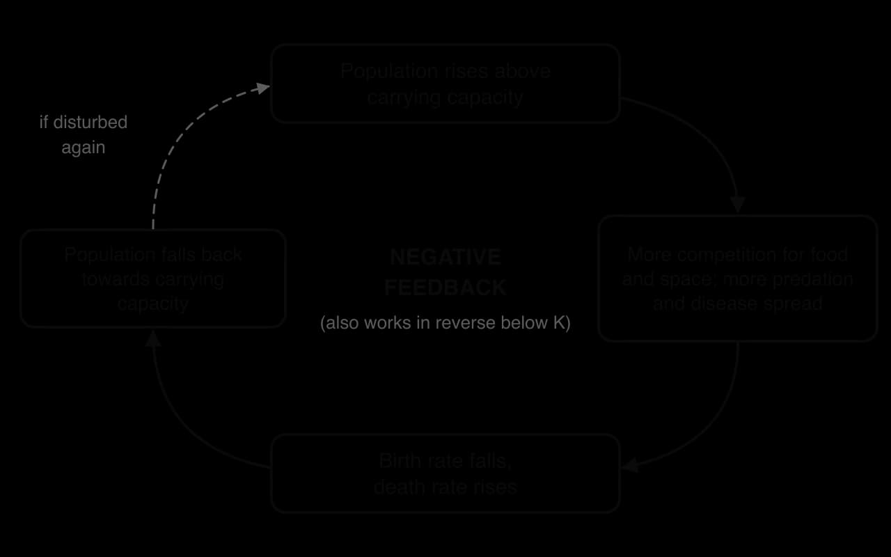
Density-dependent factors keep a population close to its carrying capacity through negative feedback, in which a change produces effects that reverse it. If numbers rise above the carrying capacity, competition, predation and disease all increase, the birth rate falls and the death rate rises, and numbers fall. If numbers fall below it, resources become plentiful, more young survive, and numbers rise again.
Population growth curves
When a few individuals arrive in a new, empty habitat with plenty of resources, their numbers rise slowly at first, because there are few of them to breed. Each generation then adds more individuals than the one before, because there are more parents. If nothing limits it, this exponential growth produces a curve that becomes steeper and steeper: a J-curve.
Real habitats are different: resources eventually start to run short. Growth slows as density-dependent factors take effect, and the population levels off around the carrying capacity. The result is an S-curve (a logistic growth curve) with four phases.
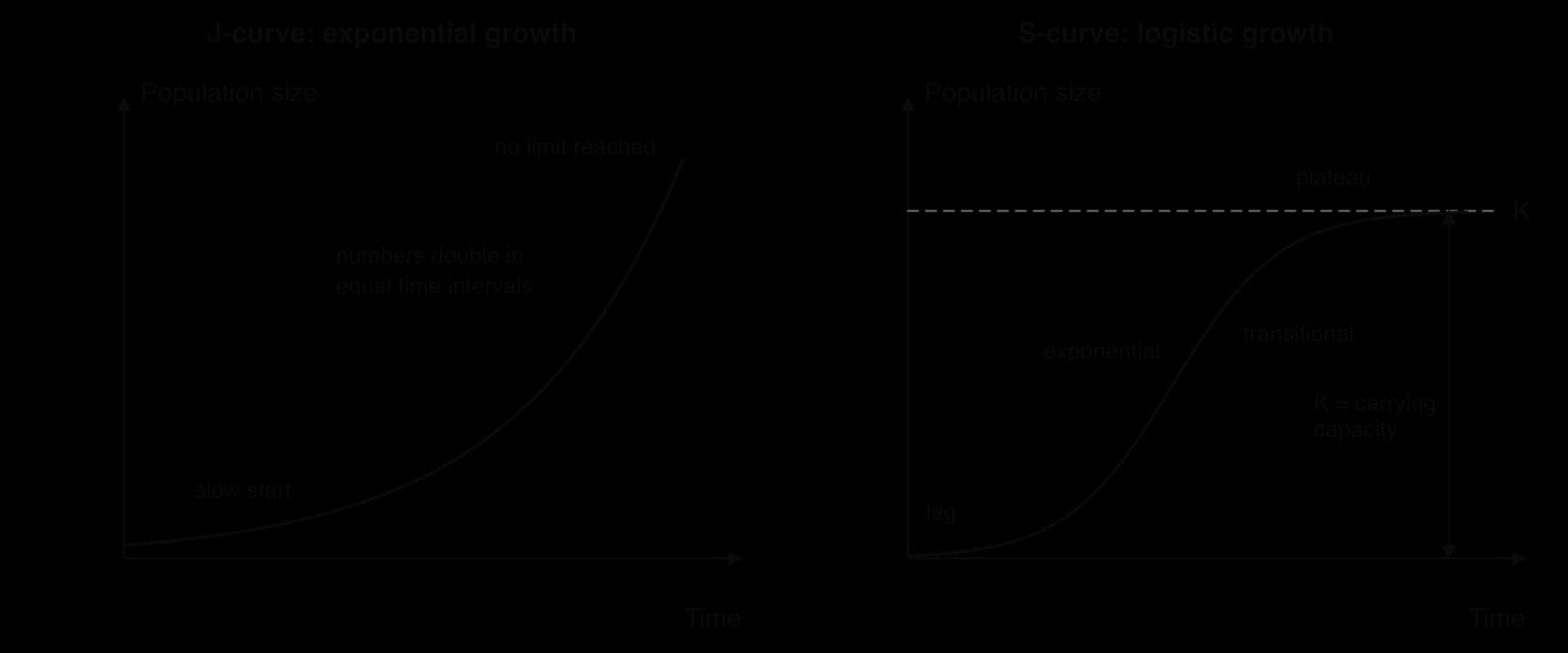
Phase of the S-curve | What happens to numbers | Why |
|---|---|---|
Lag phase | Slow growth | Few individuals; they are adjusting to the habitat and finding mates |
Exponential phase | Rapid, accelerating growth | Plenty of resources and few limiting factors; births far exceed deaths |
Transitional phase | Growth continues but slows | Resources start to run short; competition, predation and disease increase |
Plateau phase | Numbers level off and fluctuate around K | Births roughly equal deaths; density-dependent factors regulate the population by negative feedback |
Numbers and rates of change
A growth curve can be read in two ways: as the number of individuals over time, or as the rate at which that number is changing. On an S-curve the rate of growth is low in the lag phase, highest in the middle of the exponential and transitional phases, and close to zero on the plateau, where births and deaths balance. On a J-curve the rate of growth keeps increasing.
Boom and bust
Some populations do not level off smoothly. If a population grows very fast and the effects of shortage arrive late (a time lag), it can overshoot the carrying capacity and then crash. This boom and bust pattern is common when a species is introduced into a habitat without predators, or when the population damages its own resources while it is large. After the crash the population may recover and repeat the cycle, settle at a lower level, or die out.
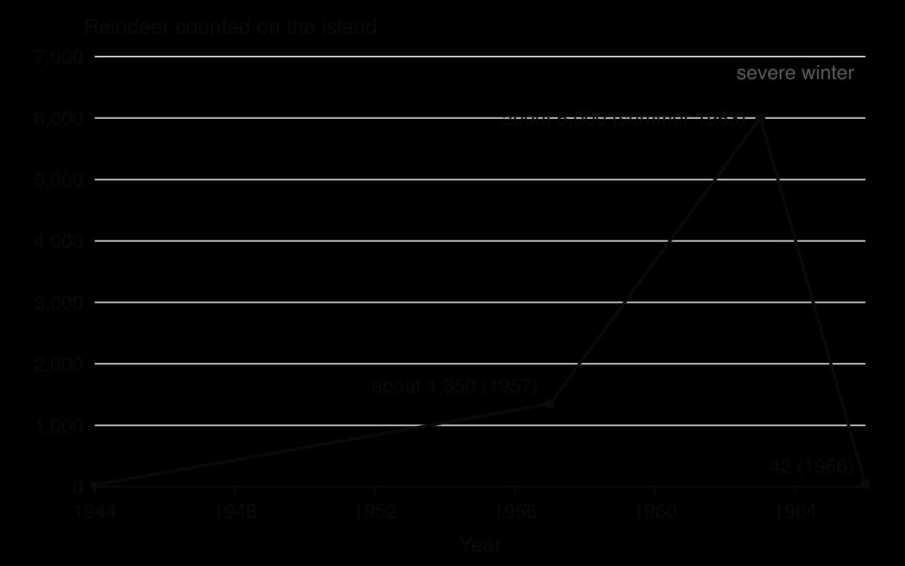
Algal blooms in nutrient-rich lakes, plagues of desert locusts after heavy rain and the reindeer of St Matthew Island in Alaska all follow this pattern. In the reindeer, numbers rose from 29 to about 6,000 in 19 years and then crashed to 42, and the extended case study traces each stage.
 YouTube
Human population and carrying capacity
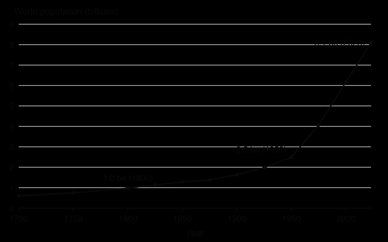
For most of history the human population grew very slowly, held back by the same factors that limit other species: food shortages, disease, war and the dangers of the environment. Over the last two centuries, many of these limiting factors have been weakened or removed. The world population passed 1 billion around 1800, reached 2.5 billion in 1950 and was about 8.1 billion in 2023.
How limiting factors have been removed
Natural predators of humans have been killed or pushed out of farmland and cities, so predation is no longer a significant cause of death.
Disease has been reduced by clean water, sanitation, vaccines and antibiotics, so death rates, especially of infants and children, have fallen.
Food supply has been increased by farming technology: machinery, irrigation, synthetic fertilisers and high-yielding crop varieties.
Space and climate limits have been overcome with housing, heating, cooling and transport, and trade moves food and resources from where they are produced to where people live.
The consequences for ecosystems are large. Feeding, housing and supplying more than 8 billion people has turned forests and grasslands into farmland, drawn down rivers and groundwater, and changed the atmosphere. Removing the limits on human numbers has often been achieved by degrading the ecosystems that support humans, so it is uncertain whether the present population, at present levels of consumption, can be sustained.
Why human carrying capacity is so hard to assess
For a reindeer population on an island, carrying capacity can be estimated from the amount of food the island produces each year. For humans, human carrying capacity is much harder to estimate, for several reasons.
The human niche is very broad and keeps changing. People eat a huge range of foods and live in every biome, from the Arctic to deserts.
Technology raises the limits. Irrigation, fertilisers, new crop varieties, desalination and renewable energy all increase what an area can supply, so any estimate is valid only for the technology of its time.
Resources move. Trade means that a city’s food, water and energy come from land and water far away, so the carrying capacity of an area cannot be judged from its own resources.
Consumption varies. The same land supports many more people eating mainly plants at a modest standard of living than people eating large amounts of meat and using a lot of energy. The answer depends on the lifestyle assumed.
Values differ. Deciding how many people the Earth “can” support means deciding what quality of life is acceptable and how much of the planet should be left for other species.
As a result, published estimates vary enormously. A 2004 review of 69 studies found estimates ranging from 0.65 billion to 98 billion people, with an average of about 7.7 billion. Meanwhile, the UN’s 2024 projections expect the world population to peak at about 10.3 billion in the 2080s and then decline slowly. A related approach compares the ecological footprint of a population with the biocapacity of the land and water available to it, which avoids a single headcount but depends on the same assumptions about consumption and technology.
Sources: Van den Bergh and Rietveld, _BioScience (2004); UN DESA, World Population Prospects (2024)._
Perspective | View of human carrying capacity | Typical response |
|---|---|---|
Technocentric | Carrying capacity is not fixed; human ingenuity will keep raising it, as it did with past technology | Invest in research: more efficient farming, clean energy, recycling of resources |
Anthropocentric | Resources should be managed so that people now and in future can live well | Sustainable development, careful management of soils, water and fisheries, slowing growth through education and health care |
Ecocentric | Humans are already beyond what the Earth can sustain and are taking space from other species | Reduce consumption, especially in rich countries; protect nature for its own sake; accept limits |
Measuring populations: sampling
Counting every plant in a meadow or every beetle in a wood is almost never possible. Instead, ecologists count organisms in a small part of the area, a sample, and use it to estimate the whole. The estimate is only as good as the sample: it must be large enough and representative of the whole area, and it must be taken in a way that avoids bias, such as choosing places that look interesting or are easy to reach.
The aim is usually to estimate abundance, the number of individuals of a species in an area, or to describe how a species is distributed. The choice of method depends on whether the organisms move, how large and how varied the area is, and what question is being asked.
Random, systematic and stratified sampling
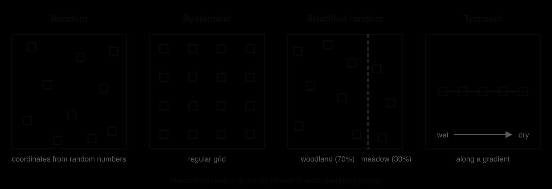
In random sampling, every point in the area has an equal chance of being chosen. A grid is laid out with two measuring tapes at right angles, and pairs of random numbers (from a calculator, a table or an app) give the coordinates of each sample. Because nobody chooses the positions, the samples are unbiased.
Systematic sampling takes samples at regular intervals: every 5 m across a field, or at every point on a grid. It is quick and gives even coverage, which is useful for mapping, but if the pattern of sampling happens to match a pattern in the habitat, such as the rows of an orchard or the ridges of a ploughed field, the results are biased.
Stratified sampling first divides the area into zones (strata) that are clearly different, such as woodland and meadow, and then takes random samples within each zone, usually in proportion to its size. This makes sure that every zone is represented, which pure random sampling might miss by chance.
Transects
Where conditions change steadily across an area, for example from the edge of a pond to dry ground, from the bottom to the top of a rocky shore, or with increasing distance from a road, the question is usually how species change along the gradient. A transect is a line laid across the area along the gradient, and samples are taken along it at regular intervals, a form of systematic sampling.
A line transect records every organism that touches the line at set intervals. It is quick but gives no information about abundance away from the line.
A belt transect places quadrats along the line, either touching each other (continuous) or at regular intervals (interrupted). It records abundance and is the usual method for studying how species change along a gradient.
Abiotic factors are measured at each sampling point at the same time, so that changes in species can be linked to changes in conditions. The results are often drawn as a kite diagram, in which the width of each band shows a species’ abundance at each point along the transect.
Method | Best used when | Strengths | Limitations |
|---|---|---|---|
Random | The area looks fairly uniform, and the aim is an average for the whole area | Unbiased; allows statistical tests | May miss small or rare zones by chance; slow in large or rough areas |
Systematic | Mapping an area or covering it evenly | Quick and simple; even coverage | Can be biased if it lines up with a pattern in the habitat |
Stratified random | The area contains clearly different zones | Every zone is represented; still random within zones | Zones must be identified first; needs the area of each zone |
Transect | Conditions change along a gradient (shore, slope, pollution source) | Shows how species and abiotic factors change together | Gives information only along the line; one transect may not be typical, so several are needed |
Quadrat sampling of non-mobile organisms
A quadrat is a square frame that marks out a standard area of ground, shore or stream bed. It is used for organisms that do not move, or move very little, such as plants, seaweeds, lichens, barnacles and limpets. Common sizes are 0.5 m × 0.5 m (0.25 m²) and 1 m × 1 m (1 m²); much larger quadrats, marked out with tapes, are used for trees. Many quadrats are divided by strings into 100 small squares to help with counting and estimating cover.

Three kinds of measurement can be taken in a quadrat, depending on the organism and the question.
Population density
Where individuals can be counted, such as daisies, limpets or young trees, the count in each quadrat gives the population density. The mean density from many quadrats is then multiplied by the total area to estimate the population size.
Percentage cover
Many plants and seaweeds grow as mats or spreading clumps in which individuals cannot be told apart, so they cannot be counted. Instead, the proportion of the quadrat area covered by the species is estimated as percentage cover. Using a quadrat divided into 100 squares, each square that is mostly covered counts as 1%. Because plants grow in layers, the cover of all species in a quadrat can add up to more than 100%.
Percentage frequency
Percentage frequency records how often a species occurs, not how much of it there is. It is the number of sampling units in which the species is present, divided by the total number of sampling units, multiplied by 100. The sampling units can be the 100 small squares of one quadrat, or a set of whole quadrats. If clover is found in 5 of 100 small squares, its percentage frequency is 5%.
Making quadrat sampling reliable
Number of quadrats. Keep adding quadrats and calculating the running mean until it stops changing much; that number is enough. In practice, ten or more per site is a common minimum.
Size of quadrat. Small enough to count accurately, large enough to contain several individuals of the species being studied.
Consistency. The same person estimating cover in every quadrat, or several people checking each other, reduces differences in judgement.
Timing. Sampling at the same season and time of day, because plants flower and animals move.
Ethics. Trampling, removing plants and disturbing animals are kept to a minimum and animals are returned to where they were found.
Sampling animals that move or hide
Animals that move, hide in leaf litter or live in water need other methods. They usually give a relative measure of abundance (more or fewer than at another site) rather than an absolute population size, unless they are combined with capture–mark–release–recapture.
Method | How it works | Organisms sampled |
|---|---|---|
Pitfall trap | A container sunk level with the soil surface, sometimes with a cover against rain; animals walking past fall in | Ground beetles, spiders, woodlice and other ground-dwelling invertebrates |
Sweep net | A strong net swept through long grass or low vegetation in a set number of sweeps | Insects and spiders on plants |
Kick sampling | The stream bed is disturbed by kicking for a set time just upstream of a net held against the current | Freshwater invertebrates such as mayfly, caddisfly and stonefly larvae |
Tullgren funnel | Soil or leaf litter is placed on a mesh under a lamp; animals move down away from the heat and light into a collecting pot | Small soil animals such as mites and springtails |
Light trap | A bright light at night attracts flying insects into a box | Moths |
Camera trap | A motion-triggered camera photographs passing animals | Mammals and ground birds; individuals can sometimes be recognised by markings |
Capture–mark–release–recapture and the Lincoln index
Estimating the size of a population of mobile animals, such as woodlice, snails, grasshoppers, fish or small mammals, cannot be done with quadrats, because the animals move in and out. The method used instead is capture–mark–release–recapture. A sample is caught, marked harmlessly and released; after the marked animals have mixed back into the population, a second sample is caught. The proportion of marked animals in the second sample is used to estimate the total population.
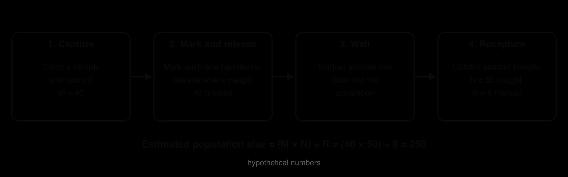
The idea behind the calculation is simple. If the marked animals have mixed evenly, the fraction of marked animals in the second sample should be the same as the fraction of marked animals in the whole population. The Lincoln index (also called the Lincoln–Petersen index) rearranges this into a formula.
M = the number of individuals caught and marked in the first sample.
N = the total number of individuals caught in the second sample (marked and unmarked).
R = the number of marked individuals recaptured in the second sample.
Assumptions of the Lincoln index
The estimate is reliable only if the population behaves as the method assumes. Each assumption, and what happens when it fails, can be used to evaluate a real study.
Assumption | If it is not true |
|---|---|
The population is closed: no births, deaths, immigration or emigration between samples | New unmarked animals dilute the marked ones, or marked animals are lost, so the estimate is wrong; keep the interval short |
Marks are not lost, and do not harm the animal or make it easier for predators to see | Fewer marked animals are recaptured (R too small), so the population is overestimated |
Marked individuals mix fully and randomly with the rest of the population | If marked animals stay near the release point, R depends on where the traps are |
Every individual has the same chance of being caught (equal catchability) | Animals that learn to avoid traps (“trap-shy”) or return for the bait (“trap-happy”) make R too small or too large |
The sampling method and effort are the same both times | A different trap number or time changes N and makes the samples not comparable |
Evaluating capture–mark–release–recapture
The method is cheap, needs little equipment and gives an absolute population estimate rather than just a relative abundance. It works best for animals that are fairly common, easy to catch and easy to mark, in an area with clear boundaries. It works poorly for very large or very small populations (few recaptures make R uncertain), for animals that move over long distances, and over long periods in which births and deaths change the population. Repeating the recapture on several days and taking a mean improves reliability.
Marking raises ethical questions. Marks must be non-toxic, must not make animals more visible to predators and must not affect movement, and handling should be brief, with animals released where they were caught. For larger animals, photographs of natural markings, such as the spots of whale sharks or the stripes of zebras, can identify individuals without capturing them at all.
Ecosystems as open systems
A community never exists on its own. Plants need light, water, carbon dioxide and mineral nutrients from soil; animals need oxygen and water; decomposers need dead matter. An ecosystem is the community together with the physical environment it interacts with, and it is the level at which energy flows and matter cycles.
Ecosystems are open systems: both energy and matter cross their boundaries. Sunlight enters and is captured by producers, and leaves as heat from respiration. Water arrives as rain and leaves as river flow and water vapour; nutrients arrive from weathering rock and leave by leaching and erosion; seeds and animals move in and out. Drawing an ecosystem as a systems diagram makes these flows visible, with storages in boxes and flows as labelled arrows.
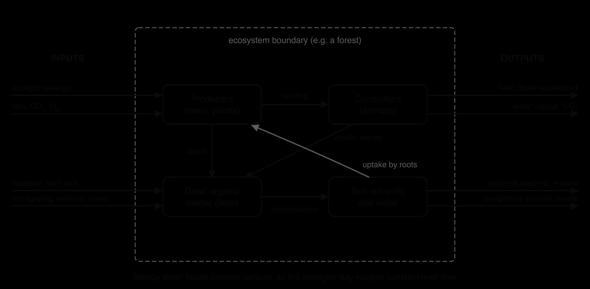
The boundaries of an ecosystem are chosen by the person studying it. A pond, a forest, a coral reef or a whole river basin can each be treated as one ecosystem. Because the boundaries are partly a choice, every ecosystem exchanges matter and energy with its neighbours, and the size of those exchanges depends on where the line is drawn.
Sustainability as a natural property of ecosystems
An undisturbed ecosystem can keep going for very long periods, because it runs on a renewable supply of energy from the Sun and recycles the matter it needs. When its inputs balance its outputs, the sizes of its storages stay roughly constant over time, even though matter and energy keep flowing through it. This is a steady-state equilibrium.
Tropical rainforests show this property clearly. Their soils are often poor, but nutrients are recycled so quickly between leaf litter, decomposers and roots that the forest supports enormous biomass and diversity, and forests of this kind have persisted in the Amazon basin for millions of years. Natural ecosystems are therefore models of sustainability: they use renewable energy, recycle almost all of their materials and produce little lasting waste.
Tipping points in ecosystems
An ecosystem in steady state is usually held there by negative feedback. Human activity can weaken these controls. If the pressure keeps increasing, the ecosystem may reach a tipping point, beyond which positive feedback takes over, the original ecosystem collapses, and a different one develops with its own new equilibrium. Returning to the original state can then be very slow or impossible, even if the pressure is removed.
The Amazon rainforest and its own rainfall
The Amazon rainforest helps to make its own rain. Trees draw water up from the soil and release it from their leaves by transpiration. Measurements of the isotopes of oxygen in rainwater, made by the Brazilian scientist Eneas Salati in the 1970s, showed that the Amazon generates about half of its own rainfall, recycling moisture five to six times as air moves westward across the basin from the Atlantic. Forests also keep transpiring through the dry season, while pastures do not.
When forest is cleared for cattle pasture and soy, or burned, less water vapour returns to the air, less rain falls downwind, and the dry season becomes longer and hotter. The remaining trees suffer drought stress, die and become more likely to burn, which removes more forest. This is a positive feedback loop.
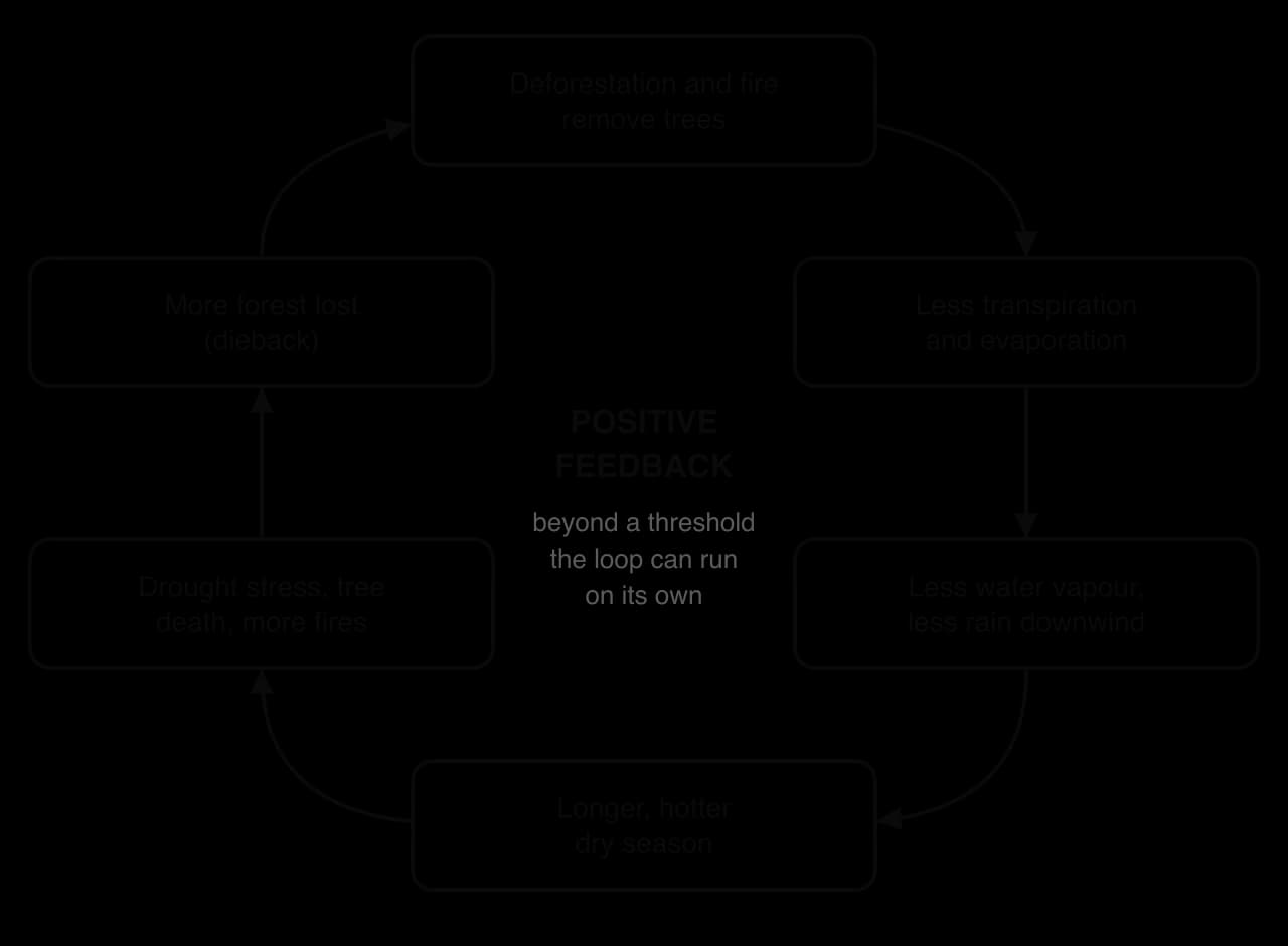
Where is the threshold? Early models suggested that the southern, eastern and central Amazon would switch towards savanna at about 40% deforestation. In 2018, Thomas Lovejoy and Carlos Nobre argued that the combined effects of deforestation, climate change and the widespread use of fire lower the tipping point to about 20–25% deforestation, and they saw the severe droughts of 2005, 2010 and 2015–16 as possible “first flickers” of it. By 2022 about 20% of the Amazon rainforest had been cleared and a further 6% was highly degraded.
Sources: Lovejoy and Nobre, _Science Advances (2018); Wikipedia, “Amazon rainforest” (read 2026)._
The exact threshold is uncertain, and scientists disagree on how close it is and whether the whole basin or only parts of it would tip. Lovejoy and Nobre’s response follows the precautionary principle: since nobody can know the precise point without crossing it, deforestation should be reduced and some cleared land restored to keep a margin of safety. Farmers and governments that depend on agricultural exports weigh these risks against income and jobs, while many Indigenous peoples of the Amazon see the forest as their home rather than a resource, and ecosystems are generally in better condition where Indigenous peoples own or manage the land.
Keystone species
In most communities, a few species have much more influence than the others. Removing them sets off changes that spread through the whole food web. The American ecologist Robert Paine introduced the term keystone species in 1969, after the central stone at the top of an arch, which holds the other stones in place.
The purple sea star on the Pacific coast
Paine worked on rocky shores in Makah Bay, on the Pacific coast of Washington State, USA. The purple or ochre sea star (Pisaster ochraceus) eats several shore animals, but especially the California mussel (Mytilus californianus), which is the strongest competitor for space on the rocks. Paine repeatedly removed every sea star from one stretch of shore and left a nearby stretch untouched.

Where the sea stars remained, about 15 species lived on the rocks. Where they had been removed, mussels spread over the space, and after three years only 8 species were left; after ten years the area was dominated by mussels alone. The sea star keeps diversity high by preventing one competitor from taking over. Since 2013, sea star wasting disease has killed huge numbers of sea stars along the Pacific coast of North America, giving an unplanned, much larger test of the same idea.
Elephants in the African savanna
African savanna elephants (Loxodonta africana) eat grasses and the leaves, bark and branches of trees, and they push over and uproot trees while feeding. This keeps woody plants from taking over and maintains the open mixture of grass and scattered trees on which grazing animals such as zebra and wildebeest depend. Where elephants have been removed, many savannas gradually turn into woodland or thicket. Elephants also disperse seeds over long distances in their dung. An animal that changes the physical structure of its habitat in this way is called an ecosystem engineer.
Sea otters in the North Pacific are another keystone species: by eating sea urchins they protect the kelp forests that urchins would otherwise graze away. African savanna elephants are now listed as Endangered, after a fall of more than half over three generations, so their loss threatens the structure of whole savanna ecosystems as well as the species itself.
Biosphere integrity and a planetary boundary
The planetary boundaries model identifies nine Earth-system processes that keep the planet in the stable conditions of the last 10,000 years, each with a boundary beyond which the risk of large, irreversible change rises. One of them is biosphere integrity: the health, diversity and functioning of life on Earth, both the variety of species and genes and the work that ecosystems do.
Ecosystem diversity and species diversity depend on each other. A varied mosaic of forests, wetlands, grasslands and reefs offers many different niches, so it supports many species; in turn, the species keep the ecosystems working by pollinating, decomposing, recycling nutrients and controlling pests. When habitats are cleared or fragmented, species lose their niche requirements and decline; when species are lost, ecosystems function less well, which can push other species towards extinction.
Evidence that the boundary has been crossed
The clearest evidence is the extinction rate. Over geological time, the background rate of extinction is estimated at about one extinction per million species per year (1 E/MSY). The planetary boundary is set at fewer than 10 E/MSY. The current rate is estimated at more than 100 E/MSY, over ten times the boundary and more than a hundred times the background rate.
Measure (control variable) | Boundary | Current estimate | Status |
|---|---|---|---|
Genetic diversity: extinction rate | Fewer than 10 E/MSY (aim about 1) | More than 100 E/MSY | Crossed |
Functional integrity: share of the net primary productivity of land taken by humans (HANPP) | Below 10% of pre-industrial net primary productivity | About 30% | Crossed |
Sources: Richardson et al., _Science Advances (2023), as summarised in Wikipedia, “Planetary boundaries” (read 2026)._
Other indicators point the same way. The 2019 global assessment of the Intergovernmental Science-Policy Platform on Biodiversity and Ecosystem Services (IPBES) estimated that around 1 million animal and plant species are threatened with extinction and that about 75% of the land surface has been significantly altered by human actions. The Living Planet Index, which tracks thousands of monitored vertebrate populations, showed an average decline of 73% in their size between 1970 and 2022 in its 2026 release. That index has been criticised because a small number of steeply declining populations strongly affect the average, so it measures trends in monitored populations, not the share of all animals lost.
Sources: IPBES Global Assessment (2019); WWF and ZSL, Living Planet Index (2026 data release).
Reversing the loss
Because biosphere integrity is connected to every other boundary (forests and oceans store carbon; wetlands clean water), its loss increases the risk of crossing other tipping points. Avoiding them means slowing and then reversing the loss of biosphere integrity, not just recording it.
Protect ecosystem integrity. Keeping whole ecosystems intact, with their structure, processes and species, slows the loss of species and keeps the niche requirements of many species met at once. Protected areas, wildlife corridors between them and the restoration of damaged habitats all do this.
Reduce the main pressures. Habitat loss, overexploitation, pollution, invasive species and climate change drive most extinctions, so reducing them helps many species at once.
Protect keystone species and ecosystem engineers, whose loss would degrade whole communities.
Set global targets. Under the Convention on Biological Diversity, countries agreed in 2022 to protect 30% of land and sea by 2030, a target known as “30 by 30”.
Views differ on how this should be done. An ecocentric view stresses protecting nature for its own sake and leaving large areas wild; an anthropocentric view stresses the services ecosystems provide to people and the need to manage them sustainably; a technocentric view looks to tools such as satellite monitoring, DNA-based surveys and the restoration of degraded land. Approaches that exclude local and Indigenous people from protected areas have also been criticised as unjust, so many recent plans give these communities a central role.
Case study: reindeer on St Matthew Island
Context
St Matthew Island is a remote, treeless island of roughly 350 km² in the Bering Sea, about 295 km north-west of Nunivak Island, Alaska, USA. Its native land mammals are only a vole and the Arctic fox; neither hunts large animals. In 1944, during the Second World War, the US Coast Guard ran a LORAN radio navigation station on the island and released 29 reindeer (Rangifer tarandus), 24 females and 5 males, all yearlings, as an emergency food supply. The station was abandoned a few years later and the reindeer were left behind.
The island’s vegetation suited reindeer well. Dry, windswept flats were covered with a thick mat of lichens, the main winter food of reindeer, while sedges, grasses and willows provided rich summer grazing. With no predators and almost no hunting, the reindeer population could grow until it reached the limits set by its food.
What happened
The biologist David Klein of the University of Alaska counted the reindeer in 1957, 1963 and 1966. In 1957 there were about 1,350, all in excellent condition: adults were heavier than reindeer in domestic herds on the mainland, and there were 75 fawns for every 100 adult females. By the summer of 1963 there were about 6,000. The lichens had been grazed, trampled and blown away, and the fawn ratio had fallen to 60 per 100 females.
The winter of 1963–64 was one of the most severe on record in the Bering Sea, with record depths of snow at weather stations nearby. With the lichens gone and deep snow covering the remaining plants, almost the entire herd starved in the late winter of 1963–64. When Klein returned in 1966, he found 42 reindeer: 41 females and a single male, with no fawns or yearlings. With so few males and no young, the population could not recover, and by the 1980s the reindeer had died out.
Data
Measure | 1957 | 1963 | 1966 |
|---|---|---|---|
Reindeer counted | about 1,350 | about 6,000 | 42 |
Density (reindeer per km²) | about 4 | about 18 | under 0.2 |
Fawns per 100 adult females (as Klein reported) | 75 | 60 | 0 |
Yearlings per 100 adult females | 45 | 26 | 0 |
Body weight of adults compared with 1957 | — | about 38% lower (females), 43% lower (males) | — |
Lichens in the winter diet | heavily grazed in places | eliminated as a significant food | — |
Sources: Klein, “The introduction, increase, and crash of reindeer on St. Matthew Island”, _Journal of Wildlife Management 32 (1968); Miller, Barry and Calvert, Rangifer Special Issue 16 (2005); Wikipedia, “St. Matthew Island” (read 2026)._
Analysis
Carrying capacity and limiting factors. Winter food (lichen) was the limiting factor. Summer forage was plentiful, which allowed rapid breeding, but the winter range set the true carrying capacity.
Missing negative feedback. On the mainland, wolves prey on reindeer and caribou, and migration lets herds move away from depleted pastures. On a small island with no predators, the only density-dependent check was food shortage, and it acted late, after the damage was done.
Time lag and overshoot. Lichens grow very slowly, so the damage to the food supply built up for years before it showed in the population. The herd kept growing into the 1960s on a food supply that was already collapsing.
A density-independent trigger. The severe winter of 1963–64, with extreme snow accumulation, killed the herd. Klein concluded that food supply, interacting with the weather, regulated the population: a smaller herd with more lichen left would probably have lost far fewer animals.
A changed ecosystem. Grazing removed lichens from the winter diet, and sedges and grasses spread into sites that lichens had occupied. Lichens grow very slowly, so this change in the vegetation could not be reversed within a few years.
Management and responses
Nobody managed the herd. After the Coast Guard left, the only reindeer removed were 105 animals shot for study or recreation, almost all between 1957 and 1963. Klein pointed out that reindeer herding at the time was seldom based on knowledge of how much grazing the range could support, and that the winter range sets the upper limit of a herd.
Introducing reindeer to islands was not unusual at the time: herds were also released on St Paul Island in the Pribilof Islands and on South Georgia in the South Atlantic, and Klein noted that the same pattern of growth and die-off had been seen in other introduced island populations. St Matthew Island is now part of the Alaska Maritime National Wildlife Refuge.
Evaluation and perspectives
Scientists still disagree about why the herd crashed. Klein saw overgrazed lichens as the root cause, with the severe winter as the trigger. In 2005, Frank Miller and colleagues re-examined his data and found that the 1957 fawn ratio had been taken from the wrong sample: about 60 fawns per 100 females were born in both 1957 and 1963, so the herd showed little sign of food shortage before the crash. In their view the extreme winter alone was decisive. Both views agree that a population with no predators grew far beyond what its winter range could support in the long term.
The case is often used as a warning about overshoot, but its lessons need care. As a test of the population models, it shows how far reality can depart from a smooth S-curve when there is a time lag and only one regulating factor. It does not show that every population will crash: most populations on the mainland, with predators, migration and many food sources, are regulated much more smoothly.
Comparisons with the human population are common but crude. Reindeer cannot change their diet, store food, trade for resources or invent new technology, whereas humans do all of these, which is exactly why human carrying capacity is so hard to assess. The case does support a narrower point that applies to humans too: a population that degrades a slowly renewing resource can keep growing for years after the damage begins, because the effects arrive with a time lag.
Perspective | How the introduction and crash look from it |
|---|---|
Anthropocentric (at the time) | Reindeer were a useful emergency food supply for people; the island’s vegetation had value only as forage |
Wildlife manager | The crash was avoidable: regular counts and harvesting could have kept the herd within the capacity of its winter range |
Ecocentric | Releasing a non-native grazer onto an island without predators harmed both the native vegetation and the animals that starved |
There is also an ethical dimension. The reindeer were introduced for human convenience, then abandoned, and almost all died of starvation. From an ecocentric point of view, deliberately introducing a species to an island without predators, with no plan to manage it, put both the reindeer and the island’s native vegetation at risk. Today, the release of non-native animals onto islands is widely recognised as one of the main causes of damage to island ecosystems.
What it shows
St Matthew Island shows carrying capacity set by a limiting resource, what happens when density-dependent regulation is weak and acts with a time lag, the difference between the S-curve model and a boom-and-bust pattern, and the interaction of density-dependent and density-independent factors. It also shows how a single introduced species can change an ecosystem: lichens were grazed out and replaced by sedges and grasses, a shift that slow lichen growth makes hard to reverse.
Clades and cladograms (HL only)
Traditional classification groups organisms by how similar they look. Modern classification aims to group them by how they are related through evolution, so that each group contains an ancestor and all of the species that evolved from it. Such a group is a clade.
Clades are found by comparing many characteristics. Physical features are used, but DNA and protein sequences are now the main evidence: the more differences have built up between the sequences of two species, the longer ago they are likely to have shared a common ancestor. Clades are nested inside each other: mammals are a clade within the larger clade of animals that lay amniotic eggs or evolved from those that did.
Reading a cladogram
A cladogram is a branching diagram that shows the probable evolutionary relationships between groups. Each branching point (node) represents a common ancestor, from which two lineages split. Groups that branch from the same node share a more recent common ancestor with each other than with any other group on the diagram.

The root at the base represents the common ancestor of every group shown.
Each node is a hypothetical common ancestor; every group to the right of a node belongs to the clade that node defines.
Features marked on a branch (such as the amniotic egg) evolved at that point and are shared by every group beyond it.
The order of names across the tips does not matter; only the pattern of branching does. Branches can be rotated around a node without changing the relationships.
Advantages of classifying by clades
It reflects evolutionary history, so groups are natural rather than based on features chosen by the classifier.
It is testable. DNA sequences provide large amounts of objective data, and new evidence can be used to test and revise a cladogram.
It improves prediction. Members of a clade share inherited genes, so a feature found in one species (a useful chemical, sensitivity to a pollutant or a disease) is likely to occur in its close relatives.
It helps conservation. Cladograms show which species represent long, separate lineages with few close relatives, so that conservation can prioritise unusual evolutionary history as well as numbers of species.
Difficulties with the traditional hierarchy (HL only)
Since Linnaeus, organisms have been placed in a hierarchy of ranked groups, each called a taxon: kingdom, phylum, class, order, family, genus and species (with a domain above the kingdom in modern schemes). Each level contains the levels below it.
Taxon | Lion | Purple sea star |
|---|---|---|
Kingdom | Animalia | Animalia |
Phylum | Chordata | Echinodermata |
Class | Mammalia | Asteroidea |
Order | Carnivora | Forcipulatida |
Family | Felidae | Asteriidae |
Genus | Panthera | Pisaster |
Species | Panthera leo | Pisaster ochraceus |
The traditional hierarchy was built before evolution was understood, mainly from visible features, and it does not always fit the branching pattern that evolution produces.
Some traditional groups are not clades. The class Reptilia traditionally included lizards, snakes, turtles and crocodiles but excluded birds. Since birds evolved from within the same lineage as crocodiles, “reptiles” in the old sense leave out some descendants of their common ancestor. The same is true of “fish”, which excludes the land vertebrates that evolved from fish.
Evolution produces branches, not fixed levels. Life has branched many times, at many different points in time, so there are far more levels of branching than the seven ranks can show. Deciding whether a group counts as an order or a family is a matter of convention.
Ranks are not equivalent. One family of insects may be tens of millions of years old and contain thousands of species, while one family of mammals may be younger and contain a few. The same rank does not mean the same amount of evolutionary difference.
Similar features can evolve independently. Distantly related organisms living in similar conditions can evolve similar shapes (convergent evolution), which can lead to them being wrongly grouped by appearance.
Genes do not always pass only from parent to offspring. Bacteria exchange genes between unrelated species, and some plants and animals form hybrids, so their relationships are networks rather than a neat tree.
Fundamental and realised niches (HL only)
A species could survive and reproduce over a wider range of conditions than it actually occupies in nature. Competitors, predators and parasites push it out of parts of that range. Ecologists therefore distinguish the fundamental niche, which a species could occupy, from the realised niche, which it actually occupies.
The difference between the two is caused by biotic interactions.
Connell’s barnacles
Two species of barnacle live on rocky shores in Scotland. On the Isle of Cumbrae, in the Firth of Clyde, the ecologist Joseph Connell found Chthamalus stellatus only on the upper shore, and Semibalanus balanoides (then called Balanus balanoides) in a band below it. Young Chthamalus settled lower on the shore too, but did not survive there. In experiments published in 1961, Connell removed Semibalanus from areas of rock. Where it was absent, Chthamalus survived much lower on the shore.
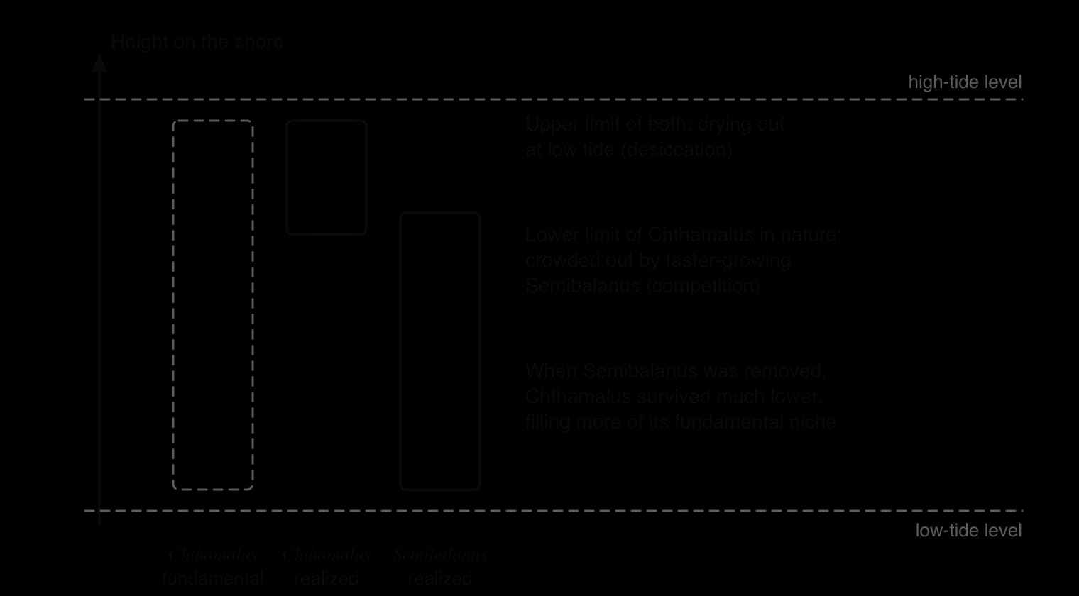
The upper limit of each species was set by an abiotic factor: how well it resists drying out when the tide is out. The lower limit of Chthamalus was set by biotic factors: Semibalanus grows faster and smothers, undercuts or crushes it, and predatory snails feed lower on the shore. The realised niche of Chthamalus is therefore much smaller than its fundamental niche.
Anoles in Florida
A more recent example shows a realised niche changing within a few years. The brown anole (Anolis sagrei), a small lizard from Cuba and the Bahamas, has spread across Florida. On small islands in Florida where brown anoles arrived, the native green anole (Anolis carolinensis) moved to higher perches in the trees, away from the competitor on and near the ground. Within about 20 generations, green anoles on these islands had evolved larger toe pads, which help them to grip on narrow, smooth perches high in the canopy.
Sources: Connell, _Ecology (1961); Stuart et al., Science (2014)._
Life cycles: r- and K-strategists (HL only)
Every life cycle involves a trade-off. An organism has a limited amount of energy and resources to spend on reproduction, so it can produce many offspring and invest little in each, or produce few and invest a great deal in each. Species near the two ends of this range are called r-strategists and K-strategists. The letters come from the equations of population growth: r is the maximum rate of increase, and K is the carrying capacity.
At the other end of the range are species that put more into each offspring.
Feature | r-strategists | K-strategists |
|---|---|---|
Number of offspring | Very many | Few |
Parental care | Little or none | A lot |
Age at first reproduction | Early | Late |
Lifespan | Short | Long |
Body size | Usually small | Usually large |
Survival of young | Low: most die young | High |
Population pattern | Rapid growth, boom and bust, often below K | Stable, close to K |
Typical environment | Unstable, newly disturbed or temporary habitats | Stable habitats, mature communities |
Examples | Dandelions and other weeds, many insects, mice, cod | Elephants, whales, great apes, oak trees |
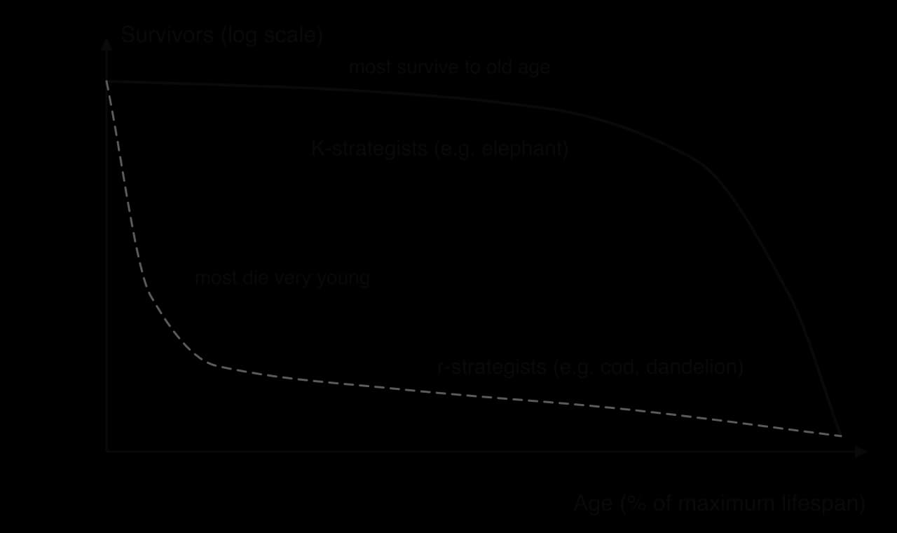
The two strategies suit different stages of succession. On newly exposed or disturbed ground, such as a landslide or an abandoned field, there is little competition, and r-strategists arrive first: their many light seeds or mobile young reach new places quickly and breed before conditions change. As a community matures and resources become fully used, K-strategists, which compete well for limited resources, gradually replace them.
The strategies also affect how species respond to human pressure. r-strategists recover quickly after a population falls and include many pests and invasive species. K-strategists recover slowly: an African savanna elephant female first ovulates at about 11 years old and then usually has a calf only every four or five years, so populations reduced by poaching take decades to rebuild.
Using ecology to understand human impacts (HL only)
Knowing how species are related, what their niches require and how their life cycles are timed makes it possible to predict which species will be most affected by human change, and why. Many life cycles are synchronised with the seasons, and with the life cycles of other species. Temperature and day length act as cues: the opening of leaves, the emergence of insects, the flowering of plants and the egg-laying of birds all happen at the time that suits them. The timing of these seasonal events is called phenology.
Phenological mismatch
Climate change can disrupt this timing. Spring events that respond mainly to temperature, such as the opening of oak leaves and the hatching of the caterpillars that feed on them, have moved earlier as springs have warmed. Events that respond to other cues, such as day length, or that depend on animals arriving from elsewhere, may not move by the same amount. When two linked life cycles shift by different amounts, the result is a phenological mismatch.
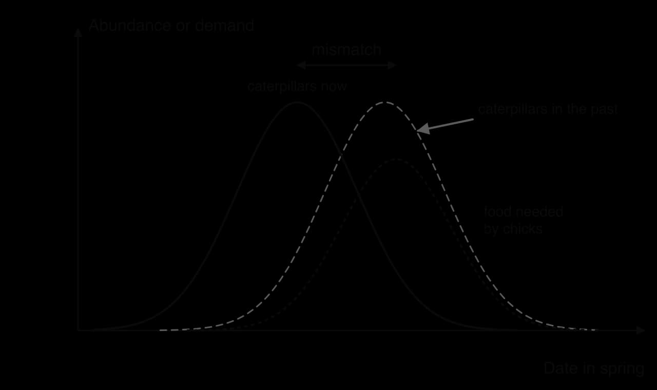
Great tits (Parus major) in Wytham Woods near Oxford, England, feed their chicks mainly on caterpillars of the winter moth (Operophtera brumata), which hatch when oak leaves open. A study of 47 years of records showed that the Wytham great tits have moved their egg-laying earlier by closely tracking spring temperatures, so they have largely kept pace with the caterpillars.
Pied flycatchers (Ficedula hypoleuca) in the Netherlands have been less able to adjust, because they spend the winter in Africa and time their return partly by day length. In areas where the food peak now comes early, their populations fell by about 90% over two decades, while populations in areas with a later food peak declined little.
Sources: Charmantier et al., _Science (2008); Both et al., Nature (2006)._
Predicting which species are most at risk
Knowledge | What it helps to predict | Example |
|---|---|---|
Classification | Related species often share sensitivities, so the impact on one suggests risks to its relatives | The chytrid fungus has hit many frog species in the same families in the Americas and Australia |
Niche requirements | Specialists with narrow niches are most vulnerable when their habitat or food changes | Koalas depend on a few eucalyptus species; pied flycatchers on a short caterpillar peak |
Life cycles | K-strategists recover slowly after losses; species with fixed timing are vulnerable to mismatch | Elephants after poaching; long-distance migratory birds under warming |
This knowledge supports better management: protecting the specific niche requirements of vulnerable species, giving slow-breeding species longer protection, and choosing which species to monitor as early warnings of change. It also shows that the effects of climate change on an ecosystem cannot be predicted from temperature alone, because they travel through the interactions between species.
Exam practice
Population and community ecology appears in every part of the assessment. Paper 2 Section A often asks for definitions, short explanations of population regulation and keystone species, and calculations such as the Lincoln index, percentage cover or population density. Paper 1 resource booklets often include field data from quadrats or transects, a population graph or a food web from an unfamiliar place, and ask for calculations, descriptions of trends and evaluation of methods. Section B essays use population growth, carrying capacity (including human carrying capacity), tipping points and biosphere integrity as the basis for extended evaluation.
Paper 2 Section A-style questions
Questions that ask for two linked things, here a distinction and an example of each, need both parts for each factor. An answer with two good definitions but no examples earns at most half the marks.
Paper 1-style data question
Paper 1 builds questions on unfamiliar data. The following resource is hypothetical, in the style of a field study on a salt marsh.
Distance from the sea (m) | 0 | 10 | 20 | 30 | 40 | 50 |
|---|---|---|---|---|---|---|
Salinity of soil water (parts per thousand) | 32 | 28 | 21 | 14 | 8 | 4 |
Cover of glasswort, Salicornia (%) | 45 | 60 | 30 | 10 | 0 | 0 |
Cover of sea purslane (%) | 0 | 10 | 40 | 55 | 25 | 5 |
Cover of grasses (%) | 0 | 0 | 5 | 30 | 70 | 90 |
Paper 2 Section B-style essay
Section B essays build from knowledge to evaluation. The final part is marked with markbands that reward breadth, well-explained examples, balance and a supported conclusion.
HL question
Summary
The biosphere is made of individuals, populations, communities and ecosystems; a species is a group that can interbreed to produce fertile offspring, and a population is the members of one species in one area at one time.
Binomial names (genus and species, in italics) and classification allow identification and prediction; dichotomous keys, reference collections, DNA barcoding and apps are used to identify organisms.
Distribution depends on abiotic factors (temperature, light, pH, salinity, dissolved oxygen, soil texture) and biotic factors; abiotic factors are measured with probes and data loggers.
A niche is the full set of conditions, resources and interactions a species depends on; habitat is where it lives.
Populations interact by herbivory, predation, parasitism, mutualism, disease and competition, with ecological, behavioural and evolutionary consequences.
Carrying capacity is set by limiting resources; density-dependent factors regulate populations around it by negative feedback, giving S-curves, while unlimited growth gives a J-curve and overshoot gives boom and bust.
Humans have removed many limiting factors, and human carrying capacity is hard to assess because of technology, trade and differing consumption.
Abundance is estimated by random, systematic, stratified or transect sampling; quadrats give density, percentage cover and percentage frequency; the Lincoln index (M × N ÷ R) estimates mobile populations under stated assumptions.
Ecosystems are open systems that can be sustainable in steady state, but human pressure can push them past tipping points, as in the Amazon moisture-recycling feedback.
Keystone species have effects far greater than their abundance; biosphere integrity is a crossed planetary boundary, shown by extinction rates over 100 E/MSY against a boundary of 10.
Clades group a common ancestor with all its descendants, and the traditional hierarchy of taxa does not always match them; species occupy realised niches smaller than their fundamental niches. (HL)
r- and K-strategists differ in offspring number, care and lifespan; knowledge of classification, niches and life cycles helps predict impacts such as phenological mismatch. (HL)
Self-check
- To do:
I can outline the levels of ecological organisation and define species, population, community, habitat and ecosystem.
- To do:
I can write a binomial name correctly and use a dichotomous key to identify an organism.
- To do:
I can describe how to measure at least three abiotic factors and explain how they affect distribution.
- To do:
I can describe the niche of a named species and give an example of each type of interaction between populations.
- To do:
I can explain carrying capacity, negative feedback and the J-, S- and boom-and-bust curves.
- To do:
I can discuss why the carrying capacity of humans is hard to assess.
- To do:
I can choose and evaluate a sampling method, and calculate density, percentage cover, percentage frequency and the Lincoln index.
- To do:
I can explain why ecosystems are open systems that can be sustainable, and describe a human-caused tipping point.
- To do:
I can explain the role of keystone species and the evidence that biosphere integrity has passed its boundary.
- To do:
I can interpret a cladogram and explain the problems with the traditional hierarchy of taxa. (HL)
- To do:
I can distinguish fundamental and realised niches, and r- and K-strategists, with named examples. (HL)
- To do:
I can explain how phenological mismatch and other human impacts can be predicted from niches and life cycles. (HL)