Notes on 4.18 Further hypothesis testing
Learning objectives
Find the critical value and critical region of a test, for a normal sample mean and for one-tailed binomial and Poisson tests.
Perform a z-test for the mean of a normal population when the population standard deviation is known.
Perform a one-sample t-test for the mean of a normal population when the population standard deviation is unknown, from raw data or from summary statistics.
Perform a paired t-test on matched pairs by treating the differences as a single sample.
Perform a one-tailed binomial test for a population proportion and a one-tailed Poisson test for a population mean.
Use technology to test the hypothesis that the population correlation coefficient is 0, and state the assumptions the test needs.
Define Type I and Type II errors and calculate their probabilities for normal, binomial and Poisson tests.
Interpret the result of a test, and the risks of each kind of error, in context.
Introduction
Subtopic 4.11, Hypothesis testing, built the logic of a test: state a null hypothesis, measure how far a sample is from what it predicts, and reject it only when a result that extreme would be rare. That logic applies to any population parameter. A food producer may want to know whether the mean mass of its loaves has fallen, a clinic whether a new drug adds hours of sleep, a quality inspector whether the proportion of faulty items has risen, a call centre whether complaints have become less frequent, and a biologist whether two measurements are correlated in the population at all.
Each of these questions uses a different distribution to calculate probabilities under the null hypothesis: the normal distribution or the t-distribution for a mean, the binomial distribution for a proportion, the Poisson distribution for a rate. The decision can be made with a p-value or with a critical region fixed in advance, and every decision carries a risk of being wrong in one of two ways. Measuring those two risks, and trading one against the other, turns a single test into a decision procedure whose reliability can be stated.
The framework and where it came from
Every test of a population parameter follows the five steps from subtopic 4.11: state the null hypothesis and the alternative hypothesis about a population parameter; choose the significance level ; find the test statistic and the p-value (or the critical region); compare; and conclude in context. Three points from that framework matter throughout.
is always an equality about a population parameter: , ,
The idea of a null hypothesis goes back to an experiment R. A. Fisher described in The Design of Experiments (1935). The phycologist Muriel Bristol claimed she could taste whether milk or tea had been poured into a cup first. She was given eight cups in random order, four of each kind, and asked to pick out the four milk-first cups. The null hypothesis is that she cannot tell the difference and is choosing at random.
The lady tasting tea as a test
There are ways to choose 4 cups from 8, and only one of them is completely correct. If she is guessing, every choice is equally likely.
Getting exactly 3 of the 4 milk-first cups right can happen in ways, so
Source: R. A. Fisher, The Design of Experiments (1935); Wikipedia article "Lady tasting tea", retrieved 2026.
Critical values and critical regions
A p-value measures how extreme one particular sample is. A different approach fixes, before any data are collected, exactly which values of the test statistic will lead to rejection. The test then becomes a rule that anyone can apply by measuring the statistic and comparing it with a boundary set in advance.
The boundary of the critical region is the critical value (or two critical values for a two-tailed test). Every other value of the statistic lies in the acceptance region.
"Acceptance" is a traditional name. A statistic in the acceptance region means only that there is not enough evidence to reject , never that has been shown to be true.
Critical regions for a sample mean
When a sample of size is taken from a normal population with mean and known standard deviation , the sample mean has the sampling distribution from subtopic 4.15.
Under , the distribution is centred at
Alternative hypothesis | Critical region | Area in each tail |
|---|---|---|
, where |
For a continuous statistic the boundary itself has probability zero, so it does not matter whether the critical region is written with or . The two methods of deciding always agree: lies in the critical region exactly when the p-value is less than , because the tail beyond
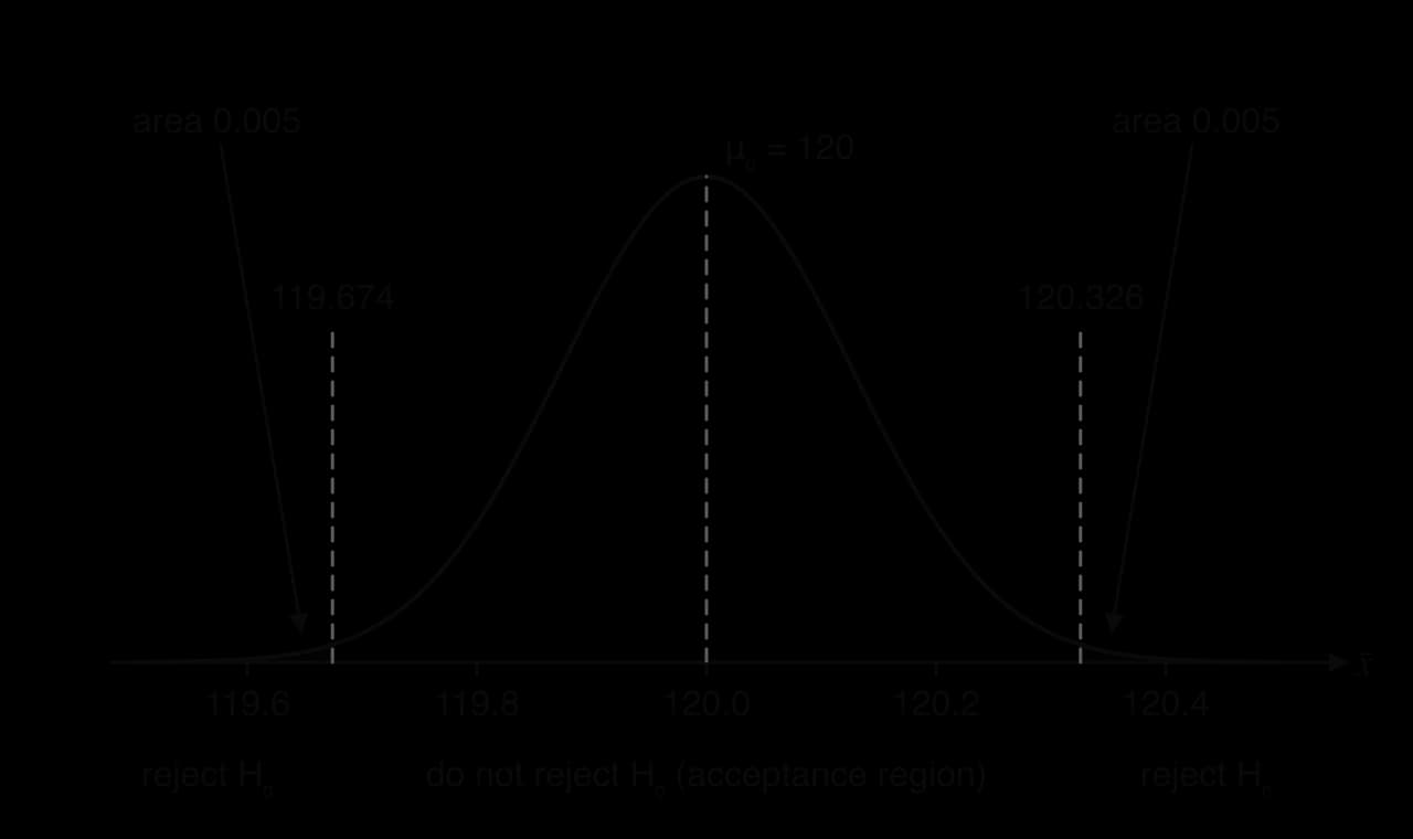
A two-tailed critical region splits between the two tails. The normal curve of for a machine part with target length 120 mm shows the result at the 1% level: each tail beyond a critical value has area 0.005, and the acceptance region in the middle holds the remaining 99%.
Critical regions for discrete distributions
A count, such as the number of clicks on a link or the number of errors in an hour, can take only whole-number values. Its probabilities jump from one value to the next, so there is usually no critical region whose probability under is exactly . The rule is to choose the largest critical region whose probability is still less than , which is the region that comes as close as possible to without going over it.
To find the boundary, list the cumulative probabilities near the tail and write down the two values either side of . For an upper-tail test the region is , where
and for a lower-tail test the region is , where
Feature | Continuous statistic () | Discrete statistic (binomial, Poisson) |
|---|---|---|
Probability of the critical region under | exactly | the largest value less than |
Tests for the mean of a normal population
A test for a single population mean compares a sample mean with a claimed value . How far apart they are only means something when measured against the standard error, and that is where the two tests differ: the standard error
Choosing between z and t
The choice depends only on whether the population standard deviation is known.
Situation | Test | Distribution of the statistic under |
|---|---|---|
known (given, or known from long experience) | z-test | standard normal, |
The rule holds whatever the sample size. A sample of 200 with unknown still uses a t-test; a sample of 5 with known still uses a z-test. For large samples the two tests give almost the same p-value, because the t-distribution approaches the normal distribution as grows, but the correct test is the one that matches what is known. Both tests assume the population is normally distributed (or, for a large sample, that the central limit theorem makes approximately normal).
The z-test
If is true and is known, standardising the sample mean gives a statistic with a fixed, known distribution.
The numerator is how far the sample mean is from the claimed mean; the denominator is how far sample means typically fall from by chance. A value of means that the sample mean is 2.26 standard errors below the claimed mean, a distance that random sampling produces rarely.
The p-value is the tail area beyond in the direction of : for
GDC procedure for a z-test
Choose the one-sample z-test: on a TI-84 Plus CE,
STAT→TESTS→Z-Test; on a Casio fx-CG50,MENU→Statistics→TEST→Z→1-SMPL.Choose data input (a list of raw values) or statistics input ( and ).
Enter ,
The written solution defines , states the hypotheses, names the test ("z-test, since is known") and gives , the p-value, the comparison with and the conclusion in context. Calculator syntax such as "Z-Test(500, 4.2, 498.1, 25)" is not mathematical notation, so it is never written in place of these.
The one-sample t-test
When is unknown it is replaced by the unbiased estimate calculated from the sample. The resulting statistic has the same structure as .
Because varies from sample to sample, varies more than would: a sample that happens to have a small
The p-value is found with the GDC's t-test, from a list of data or from , and . Critical regions are not found for t-tests: the decision is made with the p-value.
GDC procedure for a one-sample t-test
Enter the data in a list, or have , and ready.
Choose the one-sample t-test: on a TI-84 Plus CE,
STAT→TESTS→T-Test; on a Casio fx-CG50,MENU→Statistics→TEST→t→1-SMPL.Enter
The GDC's standard deviation labelled "Sx" or "sx" is , and "σx" is . A t-test entered with statistics must use
Tests from summary statistics
Data are often summarised by only , and . The unbiased estimates come first, using the methods of subtopic 4.14.
The second formula follows from
Assumptions and the link with confidence intervals
Both tests for a mean rest on three assumptions: the sample is random, the observations are independent, and the population is normal (or the sample is large enough for to be approximately normal). A volunteer sample from one class, or one shop's customers on one morning, may not represent the population at all, and then no test on the data can say anything reliable about the population mean.
A two-tailed test at significance level and a confidence interval at level give the same answer, as subtopic 4.16 shows:
Matched pairs and the paired t-test
Many studies measure the same individuals twice: blood pressure before and after a treatment, reaction time before and after training, the yield of two varieties grown side by side on the same plots. The two sets of measurements are not independent samples, because each pair shares the same person, plot or object.
Individuals differ a great deal from one another. In a reaction-time study, one person may be 50 ms slower than another whatever the conditions. Comparing two group means mixes this person-to-person variation into the comparison and can hide a real effect. Taking the difference within each pair removes everything the two measurements share, leaving only the change.
The method: one sample of differences
For each pair, calculate (the order chosen to match the claim). The differences form a single sample, and the question becomes whether their population mean is zero. A one-sample t-test on the differences answers it.
where is the number of pairs and is the unbiased estimate of the standard deviation of the differences.
The test assumes the pairs are a random sample and the differences are normally distributed; the two original variables need not be.
Case study: Student's sleep data
In 1905 the physicians A. R. Cushny and A. R. Peebles recorded the extra hours of sleep, compared with a night without medication, that 10 patients gained from each of two sleep-inducing drugs. Every patient took both drugs, so the data are matched pairs. "Student" used the data in his 1908 paper introducing the t-distribution, and they remain the textbook example of a paired test.
Patient | 1 | 2 | 3 | 4 | 5 | 6 | 7 | 8 | 9 | 10 |
|---|---|---|---|---|---|---|---|---|---|---|
Drug 1 (extra hours) | 0.7 | −1.6 | −0.2 | −1.2 | −0.1 | 3.4 | 3.7 | 0.8 | 0.0 | 2.0 |
Drug 2 (extra hours) | 1.9 | 0.8 | 1.1 | 0.1 | −0.1 | 4.4 | 5.5 | 1.6 | 4.6 | 3.4 |
= drug 2 − drug 1 | 1.2 | 2.4 | 1.3 | 1.3 | 0.0 | 1.0 | 1.8 | 0.8 | 4.6 | 1.4 |
Source: Cushny and Peebles (1905), as used by Student, Biometrika (1908); R dataset "sleep" (Rdatasets), retrieved 2026.
The table shows two things at once. The patients vary widely: patient 7 gains 3.7 hours on drug 1 while patient 2 loses 1.6 hours. Yet in every single pair except patient 5, drug 2 does better. The differences are far more consistent than the raw values, and that consistency is what the paired test measures.
Treating the same numbers as two independent samples shows why pairing matters. A pooled two-sample t-test (subtopic 4.11) compares the group means 0.75 and 2.33 hours against the large spread within each group (standard deviations 1.79 and 2.00 hours) and gives a two-tailed p-value of 0.0792, not significant even at 5%. The paired test removes the patient-to-patient variation, and the same difference in means becomes highly significant. The sample correlation between the two drugs' results is 0.795: patients who sleep well on one drug tend to sleep well on the other, which is exactly the shared variation that subtraction cancels.
The result still needs care in interpretation. Ten patients are a very small sample, the paper does not describe how they were chosen, and the differences contain one large value (4.6 hours for patient 9). The conclusion is about these drugs in patients like these, and a modern trial would use far more patients, random allocation of the order in which the drugs are taken, and a placebo.
 YouTube
The Khan Academy example shows how to recognise paired data from the design of a study and how the hypotheses change to a single mean difference.
Athlete | A | B | C | D | E | F | G | H |
|---|---|---|---|---|---|---|---|---|
Before | 312 | 287 | 345 | 298 | 331 | 276 | 305 | 320 |
After | 298 | 281 | 330 | 301 | 315 | 270 | 296 | 309 |
Reaction times of eight athletes before and after a training programme, in milliseconds (hypothetical data).
Testing a proportion: the binomial test
A claim about a population proportion , such as "85% of these seeds germinate" or "20% of visitors click the link", can be tested by counting successes in a sample of independent trials. If the claim is true, the number of successes follows a binomial distribution with the claimed proportion.
The conditions are those of the binomial model from subtopic 4.8: a fixed number of independent trials, each with the same probability of success. Binomial tests are treated as one-tailed, so is either or
The p-value method
The p-value is the probability, under , of a count at least as extreme as the one observed, in the direction of .
Observed count | p-value | |
|---|---|---|
The observed value is included in the tail, because "at least as extreme" includes the value itself. On most GDCs the binomial cumulative probability function gives only, so an upper tail is entered as
Finding a binomial critical region
A website shows a "subscribe" link to its visitors, and historically 20% of visitors click it. A redesign is meant to increase this. Under , the number of clicks from 50 visitors is
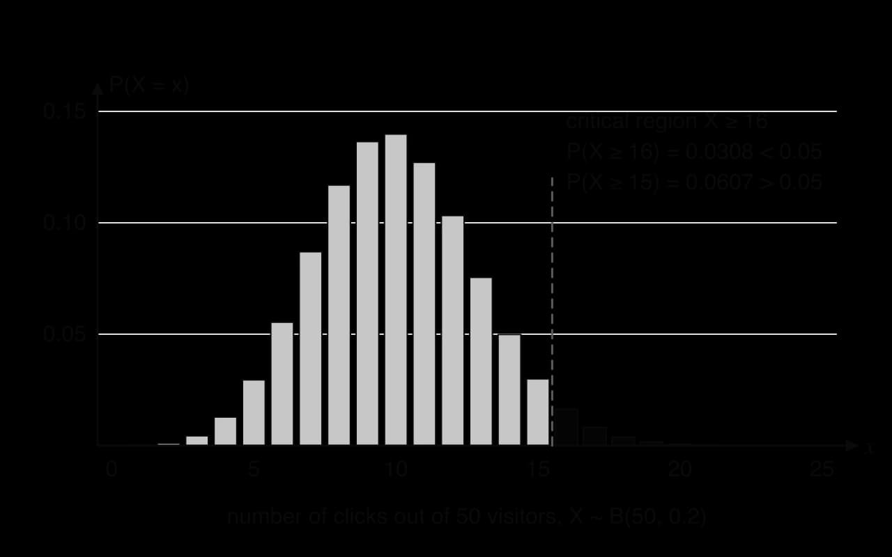
14 | 15 | 16 | 17 | 18 | |
|---|---|---|---|---|---|
0.1106 | 0.0607 | 0.0308 | 0.0144 | 0.0063 |
Upper-tail probabilities of , calculated with technology.
Testing a Poisson mean
Counts of events in an interval of time or space (calls per hour, faults per kilometre, typing errors per page) are modelled by the Poisson distribution from subtopic 4.17 when the events occur independently and at a uniform average rate. A test asks whether the mean rate has changed.
The rate in the claim is often given per unit (per minute, per day), while the count is observed over a longer interval. The mean is scaled to the interval actually observed before any probability is calculated: 3.2 complaints a day observed for 5 days gives . Like binomial tests, Poisson tests are treated as one-tailed, and the p-value and critical region rules are the same: include the observed value in the tail, and keep the probability of the critical region below .
For an upper-tail test the same scan runs the other way. The critical region is , and each upper-tail probability is found as , because the GDC's cumulative function adds probabilities from 0 upwards. Moving up by one removes a bar from the tail and lowers its probability, so the search stops at the first
Testing for correlation in a population
Subtopic 4.4 measured linear correlation in a sample with Pearson's product-moment correlation coefficient . Even if two variables are completely uncorrelated in the population, a small sample will almost never give exactly. The question for a test is whether the sample value of is far enough from 0 to show correlation in the population.
The test assumes the two variables have a particular joint distribution.
Hypotheses and the GDC test
The null hypothesis is that there is no linear correlation in the population.
The alternative is (two-tailed, any correlation), (positive correlation) or (negative correlation), chosen from the claim. A claim such as "longer hands go with longer feet" has a direction, so it gives a one-tailed test with
The GDC calculates a t-statistic from and (with ) and its p-value. The test is found in the same place as the regression t-test.
Enter the data in one list and the data in another.
Choose the linear regression t-test: on a TI-84 Plus CE,
STAT→TESTS→LinRegTTest; on a Casio fx-CG50,MENU→Statistics→TEST→t→REG.Choose the direction of ( and
Write down , the p-value, the comparison and the conclusion. Sometimes a critical value of is given instead, and the test then compares (or for a two-tailed test) with that value, as in subtopic 4.4.
Hand length (cm) | 17.2 | 18.9 | 16.5 | 19.4 | 18.1 | 17.8 | 20.2 | 16.9 | 18.6 | 19.0 |
|---|---|---|---|---|---|---|---|---|---|---|
Foot length (cm) | 23.8 | 26.1 | 24.0 | 27.3 | 24.9 | 25.8 | 27.0 | 23.1 | 26.4 | 25.2 |
Hand and foot lengths of 10 students (hypothetical data).
The scatter diagram of the hand and foot data, with the regression line , shows the elliptical cloud of points that a bivariate normal model predicts: no curvature, no outliers, and a spread of values of similar size all along the line.
When the test is not appropriate
The p-value from the GDC is meaningful only when these conditions hold, and the GDC prints a p-value whether or not they do.
Both variables are random. If one variable is chosen by the experimenter (the times days at which measurements were taken, or set doses of a fertiliser), the data are not a sample from a bivariate distribution, and the test does not apply.
The data are a random sample from the population the conclusion is about, not the whole population or a hand-picked group.
The relationship is linear. measures linear correlation only; data that follow a clear curve should be modelled, not tested for
Type I and Type II errors
A test makes a decision from a sample, so it can be wrong. There are two ways to be wrong, and they have different causes and different consequences.
A Type I error is a false alarm: the bakery is accused of underweight loaves when the mean really is 800 g. Its probability is controlled directly by the choice of critical region, because the critical region is chosen from the distribution under .
A Type II error is a missed effect: the loaves really are lighter on average, but the sample is not extreme enough to show it. The four possible outcomes of any test fit in a two-by-two table.
is true | is false | |
|---|---|---|
Reject |
A criminal trial gives a familiar comparison. The null hypothesis is "the defendant is innocent". Convicting an innocent person is a Type I error; acquitting a guilty person is a Type II error. Legal systems that demand proof "beyond reasonable doubt" choose to make Type I errors rare, and accept more Type II errors as the cost. Medical screening uses the same ideas under the names false positive (a Type I error when is "no disease") and false negative (a Type II error).
 YouTube
The jbstatistics video draws the two sampling distributions, one under and one under a specific alternative, which is exactly the picture used to calculate error probabilities.
The probability of a Type I error
A Type I error happens when is true and the statistic falls in the critical region, so its probability is the probability of the critical region calculated under .
For a test on a continuous statistic such as , this equals the significance level exactly.
For a binomial or Poisson test it equals the actual significance level, the probability of the discrete critical region, which is less than . For the web server,
The probability of a Type II error
A Type II error happens when is false and the statistic lands in the acceptance region. " is false" does not give one distribution: if the bakery's mean is not 800 g, it could be 799 g or 790 g. The probability can only be calculated for a specified alternative value of the parameter, and it must be calculated with that value.
The method has two stages. First find the critical region using the value. Then switch to the alternative value and find the probability of the acceptance region.
The two-curve diagram for the bakery shows both errors together. The solid curve is the distribution of if ; the dark tail to the left of 795.07 is the Type I error probability, 0.05. The dashed curve is the distribution if in fact ; the light area to the right of 795.07, where the test fails to reject, is the Type II error probability.

For a discrete test the method is the same, with sums of probabilities in place of areas. The critical region stays fixed, because it was chosen under ; only the distribution used to find the probability of the acceptance region changes, to the binomial or Poisson model with the true parameter.
A Poisson test is handled in the same way, after scaling the true rate to the interval of the test. The acceptance region of the web-server test is , the complement of the critical region .
Decision rules given in words
Sometimes the critical region is not derived from a significance level but stated as a practical rule, and the error probabilities measure how good the rule is. A bird survey identifies two similar species, A and B, by wingspan. Wingspans of species A are distributed cm and those of species B cm. The surveyors classify a bird as species B if its wingspan is greater than 32.5 cm.
Power and the trade-off between errors
The probability of correctly detecting a false null hypothesis has its own name.
The two error probabilities move in opposite directions. For a fixed sample, making Type I errors rarer (a smaller , a critical region pushed further into the tail) widens the acceptance region and so makes Type II errors more likely. The only way to reduce both at once is to collect more information: a larger sample shrinks the standard error
Change | Effect on | Effect on |
|---|---|---|
Smaller significance level | decreases | increases |
Larger sample size | unchanged (fixed at ) | decreases |
True value further from |
How small should be depends on the cost of each error. When a false discovery would be very costly, scientists choose a tiny significance level. Particle physicists announce a discovery only at "5 sigma", a result five standard deviations from what the null hypothesis predicts. When the ATLAS and CMS experiments at CERN announced the Higgs boson on 4 July 2012, each reported a local significance of 5 sigma, meaning a probability of less than one in three million of a result at least as strong arising by chance alone; ATLAS later reported 5.9 sigma, about 1 in 588 million.
Source: Wikipedia article "Higgs boson", retrieved 2026.
Exam focus
Further hypothesis testing appears on Paper 1 as short structured questions of 4–8 marks, on Paper 2 inside longer contextual questions, and on Paper 3 as parts of an extended investigation (often combined with a goodness of fit test, a Poisson model or a regression model). The command terms are state (the hypotheses, the distribution under , why a test is one-tailed, the type of error), find (a p-value, a critical value or region, an error probability), perform the test (which requires all of hypotheses, the statistic or p-value, the comparison and a conclusion), determine, justify and interpret.
Recurring shapes include: a binomial or Poisson test with the rate scaled to the interval; a critical region found by quoting the cumulative probabilities either side of , followed by "hence write down the probability of a Type I error"; a decision rule given in words with Type I and Type II probabilities under a stated true value; a z-test critical region for followed by a Type II error probability; a t-test from data or from and
The markscheme pattern in that question applies to every test of a mean, a proportion, a Poisson rate or a correlation: the parameter and its value in each hypothesis, the distribution named with its parameters, the probability statement for the critical value, an R1 for the comparison and an A1 for the conclusion in context that is never awarded without the R1.
Common ways marks are lost: writing as an inequality or in terms of , or the sample; leaving out part of "perform the test"; using a two-tailed p-value for a one-tailed alternative (or the reverse); using instead of
Practice questions
A fire alarm system is designed to test : there is no fire. Describe, in context, a Type I error and a Type II error, and state which is more serious, with a reason. [3]
The lengths of a species of lizard are normally distributed with standard deviation 2.5 cm. A published mean length is 50 cm. A random sample of 12 lizards from an island has mean length 51.4 cm. Test, at the 5% significance level, whether the mean length on the island differs from 50 cm. [5]
A drink is meant to contain a mean of 4.5 g of sugar per 100 ml. Seven randomly chosen bottles contain 4.9, 4.6, 5.2, 4.4, 4.8, 5.0 and 4.7 g per 100 ml. Assuming the amounts are normally distributed, perform a test at the 5% significance level of whether the mean is greater than 4.5 g. [5]
Six people's grip strengths, in kg, are measured with the right hand and the left hand.
Person | 1 | 2 | 3 | 4 | 5 | 6 |
|---|---|---|---|---|---|---|
Right | 31.2 | 28.5 | 35.0 | 26.8 | 30.1 | 33.4 |
Left | 29.8 | 28.9 | 33.1 | 25.0 | 29.5 | 31.2 |
(a) Explain why a paired test is appropriate. [1] (b) Test, at the 5% significance level, whether mean grip strength differs between the two hands. [5]
A test is carried out of against
Answers
Type I: the alarm sounds when there is no fire (false alarm). Type II: there is a fire but the alarm does not sound. The Type II error is more serious, because people may be harmed by an undetected fire, while a false alarm only causes inconvenience.
,
Summary
A critical region is the set of values of the test statistic for which is rejected; for a continuous statistic its probability under is , and for a discrete statistic it is the largest region with probability less than
Self-check
- To do:
I can write and for any test as statements about a population parameter (,