4.17 The Poisson distribution

Learning objectives

• State the conditions under which a Poisson distribution is a suitable model, in the context of a problem.

• Calculate Poisson probabilities, using the probability formula for understanding and the GDC for answers.

• Find probabilities of the form $\mathrm{P}(X < k)$, $\mathrm{P}(X \ge k)$ and $\mathrm{P}(a \le X \le b)$ correctly from a cumulative Poisson function.

• Determine the mean of a Poisson distribution for an interval of a different length or size by scaling the rate.

• Use the result $\mathrm{E}(X) = \mathrm{Var}(X) = m$, and comment on whether data with a given mean and variance could follow a Poisson distribution.

• Use the fact that the sum of two independent Poisson variables has a Poisson distribution.

• Solve problems that combine a Poisson distribution with a binomial distribution or with conditional probability, and find an unknown mean.

• Select the binomial, Poisson or normal distribution as a model for a given context, with a reason.

Introduction

Many practical questions ask how many times something happens in a fixed stretch of time or space: the number of calls reaching a help desk in a minute, the number of cars arriving at a junction in an hour, the number of typing errors on a page, the number of faults in a metre of cable. Each event happens at random, there is no fixed upper limit to the count, and yet the average number per interval is stable. The Poisson distribution is the model for counts of this kind.

The model was published by the French mathematician Siméon Denis Poisson in 1837. Ladislaus Bortkiewicz later showed in 1898 that it described the number of Prussian soldiers killed by horse kicks each year, and the Danish engineer A. K. Erlang (1878–1929) used it for calls arriving at a telephone exchange, the starting point of the modern theory of queues. Today it is used for traffic flow, hospital admissions, insurance claims, radioactive decay and genetic mutations.

YouTube

The Poisson model

Counting events in an interval

A Poisson random variable counts the number of times an event occurs in a fixed interval. The interval can be a length of time (a minute, a day, a year), a length (a metre of wire), an area (a square metre of carpet) or a volume (a litre of water). The count can be 0, 1, 2, 3 and so on with no fixed maximum, so the variable is a discrete random variable taking the values $0, 1, 2, \ldots$.

The single number $m$ describes the whole distribution, in the same way that $n$ and $p$ describe a binomial distribution. It is the average count in the interval being studied, which makes it a rate.

Some books and websites use $\lambda$ instead of $m$ for the parameter, and the two letters mean the same thing.

The conditions for a Poisson model

A count follows a Poisson distribution only when the events happen "at random" in a precise sense. Two conditions must hold.

1. Independence. Events occur independently of one another: one occurrence does not make another more or less likely, and the number of events in one interval does not affect the number in any other non-overlapping interval.

2. Uniform average rate. Events occur at a constant average rate throughout the period (or region) of interest, so that the mean number of events in an interval is proportional to the size of the interval.

A third, practical condition is usually implied: events occur singly, so two events cannot happen at exactly the same instant or point. Together the conditions describe events scattered at random, with no pattern, clustering or regular spacing.

Each condition has to be judged in the context. Calls to a taxi firm on a Friday evening may be roughly independent, but the rate is far higher at 11 p.m. than at 7 p.m., so a single Poisson model for the whole evening fails the uniform rate condition; one for the hour from 9 p.m. to 10 p.m. may be reasonable. Visitors arriving at a museum in coach parties are not independent, because one arrival brings forty more at the same moment. Goals in a football match are often modelled as Poisson, but a team that falls behind may attack harder, which challenges both conditions.

Poisson probabilities

The probability formula

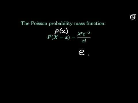
The probabilities of a Poisson distribution are given by a formula involving the number $\mathrm{e} \approx 2.718$ and the factorial function.

For $X \sim \mathrm{Po}(m)$,

Three features of the formula are worth knowing. For $x = 0$ it gives $\mathrm{P}(X = 0) = \mathrm{e}^{-m}$, the probability of no events at all, which is needed whenever an event must not happen in an interval. Each probability is the previous one multiplied by $\frac{m}{x}$

The shape of a Poisson distribution

The shape depends only on $m$. For small $m$ the most likely count is 0 and the distribution is strongly skewed to the right, with a long tail of rare larger counts. As $m$ increases, the peak moves to the right and the distribution becomes more symmetric. The bar charts of $\mathrm{Po}(0.5)$, $\mathrm{Po}(2)$, $\mathrm{Po}(5)$

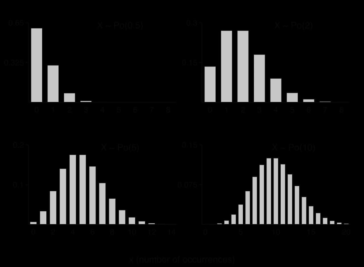
For large $m$ the shape looks increasingly like a normal distribution with mean $m$ and variance $m$. The counts remain whole numbers, however, and the GDC calculates Poisson probabilities exactly for any $m$, so the Poisson model itself should be used.

Calculating probabilities with the GDC

Probability and cumulative functions

The GDC has two Poisson functions. The Poisson probability function gives $\mathrm{P}(X = x)$ for a single value. The Poisson cumulative function gives $\mathrm{P}(X \le x)$, the cumulative probability of $x$ or fewer events. On a TI-84 Plus CE they are poissonpdf and poissoncdf (2nd VARS for the distribution menu); on a Casio fx-CG50 they are Ppd and Pcd (MENU → Statistics → DIST → POISSON). Each needs the mean $m$

Because a Poisson variable takes only whole-number values, every inequality must be turned into one of the form $\mathrm{P}(X \le k)$ before the cumulative function is used. The strict and non-strict inequalities give different answers.

Writing out the values that are included ("at least 8 means 8, 9, 10, …, so the complement is 7 or fewer") before using the cumulative function prevents most errors.

What to write down

The GDC does the arithmetic, but the working must show the model and the probability statement in mathematical notation:

1. Define the variable in words: "Let $X$ be the number of cars passing in 10 minutes."

2. State its distribution with the parameter: $X \sim \mathrm{Po}(6.2)$.

3. Write the probability required and, if needed, its rewritten form: $\mathrm{P}(X \ge 8) = 1 - \mathrm{P}(X \le 7)$

Calculator syntax such as poissoncdf(6.2, 7) is not mathematical notation and does not show the model.

Scaling the mean to the interval

Under the uniform rate condition, the mean number of events is proportional to the size of the interval. If calls arrive at a mean rate of 3 per minute, the mean in 5 minutes is $5 \times 3 = 15$, and the mean in 20 seconds is $\frac{1}{3} \times 3 = 1$

Area and length scale in the same way. Faults that occur at a mean rate of 0.3 per 10 m² of carpet occur at a mean of 1.2 per 40 m², because 40 m² is four times as large.

Biological mutation gives an example of a very small rate per unit applied over a large interval. The genome of HIV has about 10,000 base pairs, and copying introduces about 1 mutation per 30,000 base pairs, so the number of mutations in one replication is modelled by $\mathrm{Po}\left(\frac{10\,000}{30\,000}\right) = \mathrm{Po}\left(\frac{1}{3}\right)$

Source: mutation rate and genome length as given in Wikipedia, "Poisson distribution", accessed 2026.

Rates that change

When the rate changes during the period, the model is applied separately to intervals in which the rate is constant. If a website receives a mean of 40 visits an hour during the day and 10 an hour overnight, the number of visits between 18:00 and 22:00, when the daytime rate applies until 20:00 and the overnight rate after it, has mean $2 \times 40 + 2 \times 10 = 100$, and it is still Poisson because counts in separate intervals are independent and the sum of independent Poisson counts is again Poisson (the additive property of the Poisson distribution). A single rate of 25 an hour applied to any interval would give wrong answers whenever the interval was not an even mix of the two periods.

Mean and variance

E(X) = Var(X) = m

The mean and the variance of a Poisson distribution are equal.

The binomial origin of the distribution makes them reasonable. For $\mathrm{B}(n, p)$ with $np = m$, the expected value is $np = m$ and the variance is $np(1 - p) = m\left(1 - \frac{m}{n}\right)$

The equal mean and variance means that the spread of a Poisson count grows with its mean, but more slowly. For $\mathrm{Po}(4)$ the standard deviation is 2, half the mean; for $\mathrm{Po}(100)$ it is 10, a tenth of the mean, so large counts are relatively more predictable than small ones.

Mean and variance as evidence for a Poisson model

Because a Poisson distribution has equal mean and variance, a set of counts whose sample mean and sample variance are close supports a Poisson model; a variance much larger than the mean counts against it. The check is quick: calculate both from the data with the GDC's one-variable statistics (values in one list, frequencies in another), then compare.

Overdispersion usually means that one of the conditions fails. If the rate varies (busy days and quiet days mixed together), or events come in clusters (one accident causing a second), the counts spread out more than a Poisson model allows. A variance much smaller than the mean (underdispersion) suggests events that are more regular than random, such as appointments booked at fixed times.

The 2022 FIFA World Cup gives a real test. The frequency table shows the number of goals (including extra time, excluding penalty shoot-outs) in each of the tournament's 64 matches.

Source: openfootball worldcup.json (2022 match results), checked against the tournament total of 172 goals in Wikipedia, "2022 FIFA World Cup", accessed 2026.

Adding independent Poisson variables

The additive property

If two different kinds of event each occur at random, at their own constant rates and independently of each other, then the events of either kind together also occur at random, at a rate equal to the sum of the two rates. This gives a simple rule for counts.

The rule extends to any number of independent Poisson variables: their sum is Poisson with mean equal to the sum of the means. Scaling the mean to a longer interval is a special case, because the count in 3 months is the sum of three independent monthly counts.

Independence is essential. The number of passengers getting on a bus and the number getting off at the same stop are not independent of the bus's crowding, so their sum need not be Poisson.

Sums of counts and multiples of a count

The count in 2 hours is $X_1 + X_2$, the sum of two independent hourly counts, and it is Poisson with mean $2m$. The variable $2X$, twice a single hour's count, is different: it can only take even values, and its variance is $2^2\,\mathrm{Var}(X) = 4m$

Problems that combine distributions

Poisson followed by binomial

Many problems use a Poisson probability as the probability of "success" in a second, binomial, stage. If each day independently has probability $p$ of no complaints to a shop, then the number of days out of 30 with no complaints is $\mathrm{B}(30, p)$. The sign of this structure is a question about how many intervals (rooms, days, rolls, weeks) have some property, out of a fixed number of intervals.

The expected number of intervals with a property is the number of intervals multiplied by the probability. A reader who borrows a mean of 1.5 books a week will, on average, have $52 \times \mathrm{P}(X \ge 3) = 52 \times 0.191 = 9.94$ weeks a year in which at least 3 books are borrowed.

Several intervals with different requirements

When a problem specifies what happens in each of several intervals separately ("complaints on the first and third days only"), the probability is the product of the separate probabilities, by independence of counts in non-overlapping intervals. With a daily count $X \sim \mathrm{Po}(m)$, "at least one complaint on days 1 and 3 and none on day 2" has probability $\mathrm{P}(X \ge 1) \times \mathrm{P}(X = 0) \times \mathrm{P}(X \ge 1)$

Conditional probabilities

Conditional probability questions use $\mathrm{P}(A \mid B) = \frac{\mathrm{P}(A \cap B)}{\mathrm{P}(B)}$ as in subtopic 4.6. With counts, the event $A \cap B$

Finding an unknown mean or number

Solving for m

When a probability is given and the mean is unknown, the equation is solved for $m$. The probability of no events is the simplest case, because $\mathrm{P}(X = 0) = \mathrm{e}^{-m}$ can be solved with a logarithm. Other cases are solved with the GDC: graph the cumulative probability as a function of $m$ and find where it meets the given value, or use the equation solver.

The least number of sources

A harder type of problem asks for the least number of independent sources needed for the total count to reach some probability. With $n$ sources each $\mathrm{Po}(m)$, the total is $\mathrm{Po}(nm)$, and a table of values of the probability for successive $n$ gives the answer.

Choosing between the binomial, Poisson and normal distributions

Three standard distributions are now available, and the choice between them has to be made from the context and justified.

The decisive question is usually whether there is a fixed number of trials. "Of 20 patients, how many recover?" has 20 trials, so it is binomial. "How many patients arrive in an hour?" has no fixed number of possible arrivals, so it is Poisson if arrivals are independent at a constant rate. "How long does a patient wait?" is a continuous measurement, so it may be normal. For a Bernoulli trial setting with very many trials and a very small probability, the binomial and Poisson models agree closely, and either may be used.

YouTube

Case study: Flying-bomb hits on south London

In the summer of 1944, V-1 flying bombs were launched at London. Many Londoners believed that the bombs were landing in clusters, which would have meant that they were being aimed accurately at particular targets. In 1946 the actuary R. D. Clarke tested the belief with a Poisson model. He chose an area of 144 square kilometres of south London where the overall density of hits was nearly constant, divided it into 576 squares of a quarter of a square kilometre, and counted the number of bombs that landed in each square. In total 537 bombs fell in the area.

If the bombs fell at random, the hits in each square are independent events with a uniform average rate across the area, so the number of hits in a square should follow a Poisson distribution with mean

The expected number of squares with $x$ hits is $576 \times \mathrm{P}(X = x)$ for $X \sim \mathrm{Po}(0.932)$. For example, the expected number of squares with no hits is $576 \times \mathrm{e}^{-0.932} = 226.74$

Source: R. D. Clarke (1946), "An application of the Poisson distribution", Journal of the Institute of Actuaries 72, 481.

The observed and expected numbers agree closely in every column, as the paired bar chart shows.

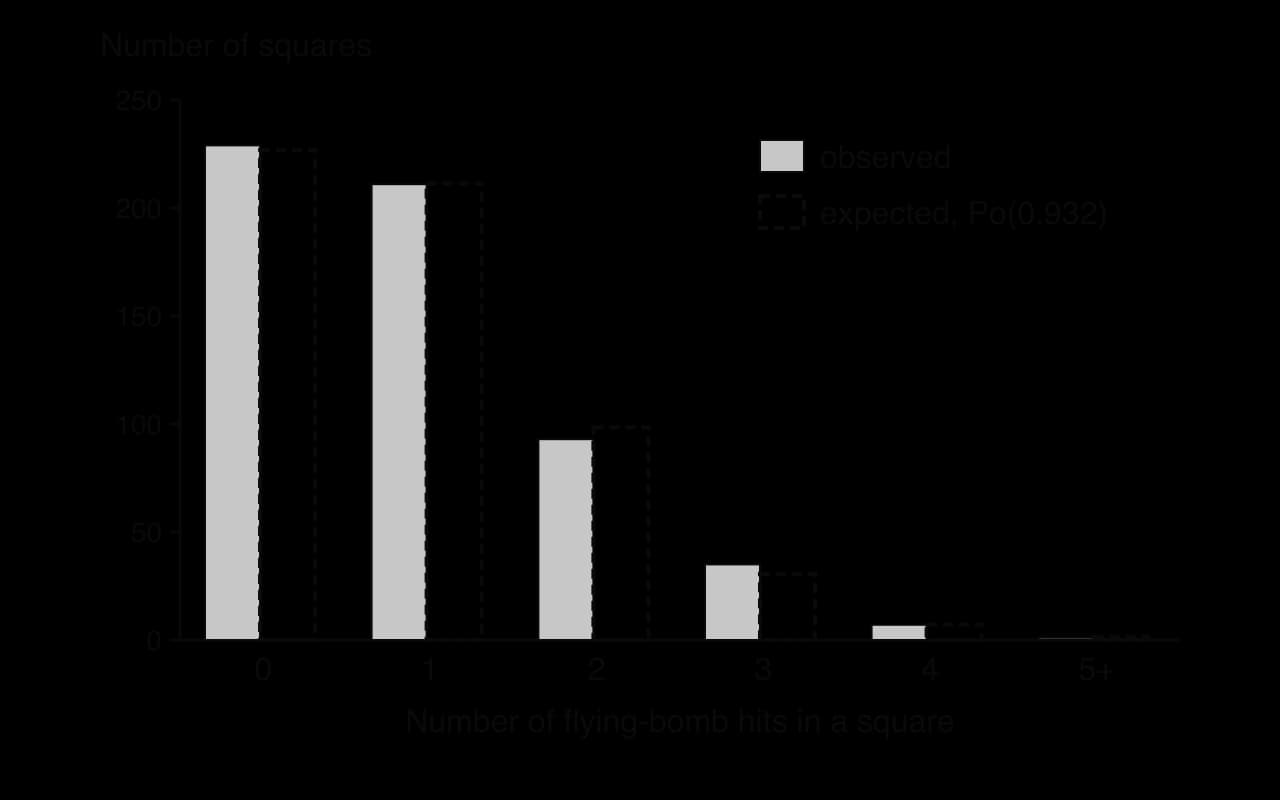
Clustering would have shown up as too many empty squares together with too many squares hit several times, which is overdispersion. The observed counts show no such excess. Since the square with "5 or more" hits must contain 7 (the total is 537), the sample variance of the counts can also be found: it is 0.969 with divisor $n$, very close to the mean 0.932. Clarke concluded with a chi-squared test that the hits were consistent with random scatter; that test, with the mean estimated from the data, is the subject of subtopic 4.12. A goodness of fit test gives evidence, not proof, and later re-analyses of the wider region have suggested that hits were denser in some parts of south London than others, so the uniform rate holds only within the carefully chosen area.

The case study shows both the strengths and the limits of the model. The apparent clusters people saw were what randomness produces: with 576 squares, a handful of squares hit four or more times is expected even when no square is targeted. The conclusion depends on the uniform-rate assumption, which is why Clarke restricted the analysis to an area where it was plausible.

Exam focus

The Poisson distribution appears often, in short Paper 1 questions of 2–6 marks and as parts of Paper 2 questions, frequently linked to a binomial stage, conditional probability, or a test or error probability from subtopic 4.18. Paper 3 may use it within a longer investigation, for example to justify a model from the mean and variance of data before a goodness of fit test. Common command terms are find, calculate, write down, state (an assumption or a distribution), determine and hence state why.

Marks are typically (M1) or (A1) for the scaled mean and the stated distribution, (M1) for a correct conversion of an inequality, A1 for the answer, and (M1)(A1) for recognising a binomial stage with the correct parameters. Assumptions earn credit only when they are precise and in context.

Marks in Poisson questions follow a fixed sequence: define the variable, state the distribution with the scaled mean, write the probability in correct notation, then use the GDC. A binomial layer is recognised by a fixed number of intervals in which some property is counted.

Practice questions

1. $X \sim \mathrm{Po}(5.3)$. Write down $\mathrm{E}(X)$, $\mathrm{Var}(X)$ and the standard deviation of $X$. [2]

(a) Find the mean and variance of the number of customers per minute. [2] (b) Comment on whether a Poisson model is suitable. [1]

9. $X \sim \mathrm{Po}(2.5)$. Find $\mathrm{P}(X \le 4 \mid X \ge 2)$. [4]

10. For each context, state whether a binomial, Poisson or normal model is most suitable, with a reason: (a) the number of earthquakes of magnitude 6 or more in a region in a year; (b) the number of heads in 50 tosses of a coin; (c) the lifetime of a light bulb. [3]

Summary

• $X \sim \mathrm{Po}(m)$ models the number of events in a fixed interval of time or space when events occur independently and at a uniform average rate; $m$ is the mean number in that interval.

• $\mathrm{P}(X = x) = \dfrac{\mathrm{e}^{-m}m^x}{x!}$

Self-check

• To do:

  I can state the two Poisson conditions in the context of a question, precisely.

• To do:

  I can explain why a varying rate or clustered events make a Poisson model unsuitable.

• To do:

  I can use the formula $\frac{\mathrm{e}^{-m}m^x}{x!}$