4.19 Transition matrices and Markov chains

Learning objectives

• Draw a transition diagram for a system that moves between a finite number of states, and complete one from a description.

• Write down a transition matrix in which each column holds the probabilities of moving from one state, and interpret any entry in context.

• Write down an initial state vector of probabilities or of numbers in each state.

• Calculate the state vector after $n$ steps with $\boldsymbol{s}_n = T^n\boldsymbol{s}_0$, using the correct number of steps.

• Interpret the entries of a power $T^n$ as probabilities of moving between states in exactly $n$ steps.

• Determine whether a Markov chain is regular, and explain what regularity guarantees about the long term.

• Find the steady state by raising the transition matrix to a high power, by solving a system of linear equations, and as the eigenvector for the eigenvalue 1 scaled so that its entries sum to 1.

• Give steady-state and long-term probabilities exactly when asked, as fractions or from an eigenvector with integer entries.

• Describe the long-term behaviour of a chain with an absorbing state.

Introduction

Many systems move step by step between a small number of conditions: a day is dry or wet, a customer uses one company or another, a shared bike sits at one of several docking stations, a gambler holds a certain amount of money. When the chance of each move depends only on the present condition, the system can be modelled by a Markov chain. A square table of probabilities, the transition matrix, then turns every question about the future into matrix multiplication, and the long-run behaviour of the system appears as a fixed vector that the matrix leaves unchanged.

Markov chains are used to model weather, the spread of customers between competing firms, the position of a random web surfer, the letters of a language and the moves of a board game. The method draws together probability from subtopics 4.5 and 4.6, matrices from subtopic 1.14 and eigenvectors from subtopic 1.15.

States, Markov chains and the Markov property

States

The first step in any Markov model is to list the conditions the system can be in. For a model of the weather in a town, a simple choice is "dry" and "wet" for each day. For a bike-share scheme, it is the docking station at which a bike ends the day. Every observation of the system must fall into exactly one of these conditions, called states.

Choosing the states is a modelling decision. Splitting the weather into "dry", "light rain" and "heavy rain" gives a more detailed model with three states and nine transition probabilities to estimate instead of four. More states describe the system more closely but need more data to estimate their probabilities.

The Markov property

A sequence of states observed at equal steps (days, months, turns of a game) is a chain. In general, the probability of the next state could depend on the whole history: whether it rained yesterday, the day before and the day before that. The simplest useful model assumes that only the present state matters.

With the Markov property, a forecast for tomorrow needs only today's weather. This is an assumption about the system, and real systems satisfy it only approximately: a run of wet days might make another wet day more likely than one wet day alone would. A model that ignores such effects can still describe the long-run proportions well; Markov's chain of vowels and consonants in a Russian novel is an example.

The second condition in the definition, that the probabilities do not change from step to step, matters as much as the first. A chain in which the chance of rain after a dry day is 0.2 in winter and 0.1 in summer would need a different model for each season.

Transition probabilities and transition diagrams

Transition probabilities

Suppose that in a town (a hypothetical model), a dry day is followed by another dry day with probability 0.8 and by a wet day with probability 0.2. A wet day is followed by a dry day with probability 0.4 and by a wet day with probability 0.6. Each of these four numbers is a conditional probability: the probability of tomorrow's state given today's state.

From any one state, the system must go somewhere at the next step, even if "somewhere" is the same state. The transition probabilities out of each state therefore add up to 1: from a dry day, $0.8 + 0.2 = 1$; from a wet day, $0.4 + 0.6 = 1$. Checking these sums is a quick way to find a probability that has been misread or left out.

Transition diagrams

A diagram shows the states and the possible moves at a glance. Each state is drawn as a circle, and each possible move as an arrow labelled with its probability. A move that keeps the system in the same state is drawn as a loop.

The transition diagram of the weather model has two states, two loops and two arrows between the states.

A transition diagram is a directed graph in the sense of subtopic 3.14: the direction of each arrow matters, because the chance of a wet day after a dry one (0.2) differs from the chance of a dry day after a wet one (0.4). An arrow with probability 0 is simply left out.

YouTube

A three-state example

A bike-share scheme in a small city (hypothetical) has docking stations at a park, a harbour and a university. Records show where a bike that starts the day at each station ends the day.

• From the Park: 60% end at the Park, 30% at the Harbour, 10% at the University.

• From the Harbour: 20% end at the Park, 70% at the Harbour, 10% at the University.

• From the University: 25% end at the Park, 15% at the Harbour, 60% at the University.

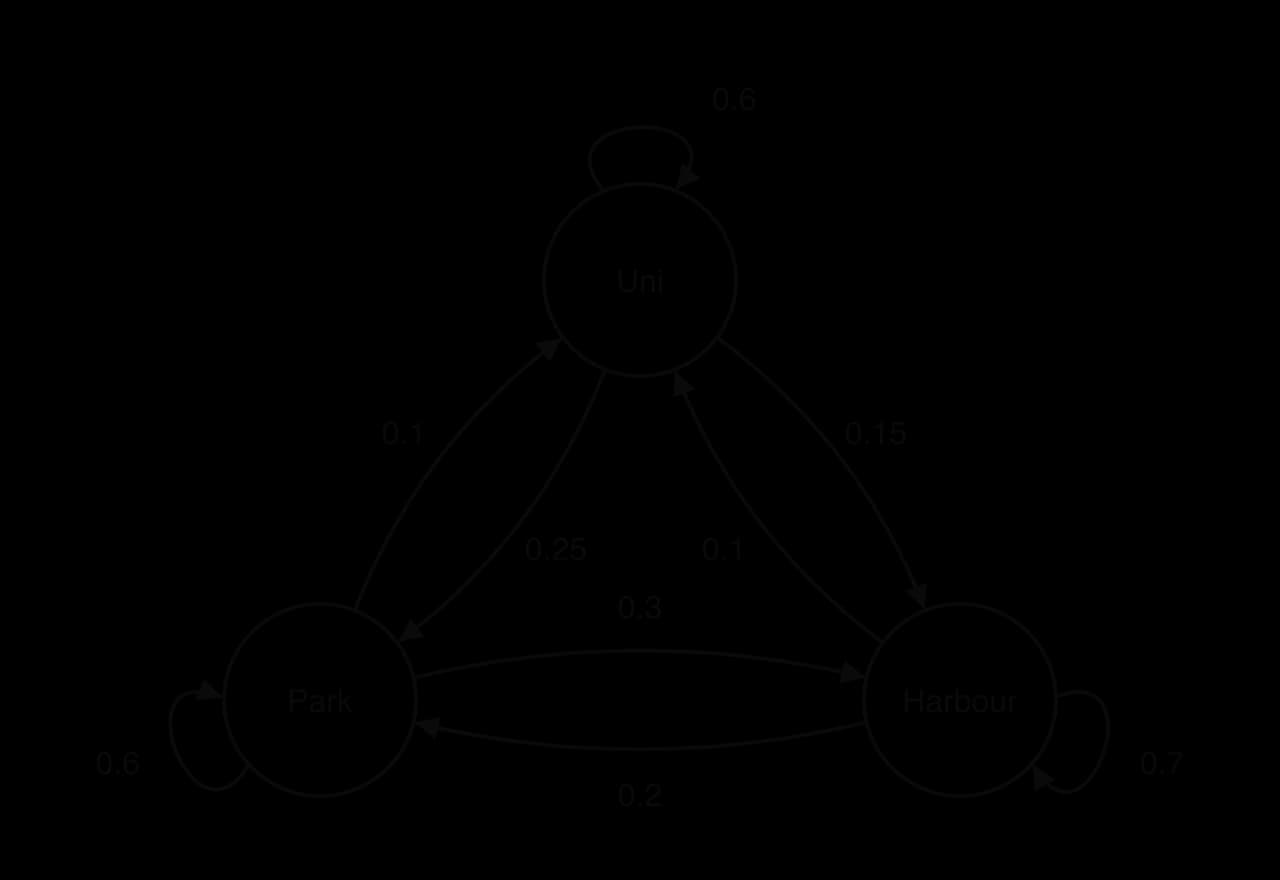
The diagram makes it easy to see that bikes drift towards the Harbour: it keeps 70% of its own bikes and receives 30% of the Park's. Whether this means the Harbour eventually holds most of the bikes depends on all nine numbers together, which is the question the steady state answers.

Transition matrices

Building the matrix: column = from, row = to

The transition probabilities are stored in a square matrix with one row and one column for each state, listed in the same order. The standard convention is that each column describes where the system goes from one state: column $j$ holds the probabilities of moving from state $j$, and the entry in row $i$ of that column is the probability of moving to state $i$.

For the weather model, with the states in the order dry, wet, the matrix with labels is:

Writing "from" across the top and "to" down the side before filling in any numbers prevents the most common error. Each column is one state's set of outgoing probabilities, so each column sums to 1: $0.8 + 0.2 = 1$ and $0.4 + 0.6 = 1$. The rows have no such rule: the first row, $0.8 + 0.4 = 1.2$

For the bike-share scheme, in the order Park, Harbour, University:

Column 1 holds the three percentages for bikes starting at the Park, column 2 those starting at the Harbour, and column 3 those starting at the University. Each column sums to 1.

The transposed convention

Some textbooks and websites write transition matrices the other way round, with rows summing to 1 and the state written as a row vector multiplied on the left. Both conventions describe the same chain and give the same answers if one of them is used consistently, with $\boldsymbol{s}_n^{\mathsf{T}} = \boldsymbol{s}_0^{\mathsf{T}}(T^{\mathsf{T}})^n$

Matrices with unknown entries

Because each column sums to 1, a transition matrix with some entries missing can often be completed. Each column with one unknown entry gives that entry at once. Interpreting the entry then needs the convention: an entry's column is where the system comes from and its row is where it goes to.

State vectors and the first step

Initial state vectors

The transition matrix describes how the system moves; a second object is needed to describe where it is. A state vector is a column vector with one entry for each state, in the same order as the rows and columns of $T$.

The entries can be probabilities, in which case they add up to 1, or numbers of people or objects, in which case they add up to the total population being modelled. The same matrix works for both, because multiplying a vector of counts by $T$ moves each fraction of each group to its new state.

A known starting state gives a vector with a single 1 and 0s elsewhere. An uncertain start, such as "a 30% chance that today is wet", gives $\begin{pmatrix} 0.7 \\ 0.3 \end{pmatrix}$. A count start, such as 150 bikes at the Park, 100 at the Harbour and 50 at the University, gives $\begin{pmatrix} 150 \\ 100 \\ 50 \end{pmatrix}$

Why one step is a matrix multiplication

Suppose today is dry with probability $d_0$ and wet with probability $w_0$. Tomorrow can be dry in two ways: today dry and stays dry, or today wet and turns dry. These two routes are mutually exclusive, so, as with the branches of a tree diagram, their probabilities are multiplied along each route and added across routes.

The two equations are exactly the rows of a matrix multiplication:

This is why the column convention is used. Row $i$ of $T$ collects every probability of arriving at state $i$, one from each starting state, and the row-by-column product weights each by the probability of being in that starting state. The order of the product matters: $T\boldsymbol{s}_0$ is a column vector, while $\boldsymbol{s}_0 T$

Powers of transition matrices

Several steps: sₙ = Tⁿs₀

Each step multiplies the state vector by $T$ once more, so the steps chain together:

Continuing in the same way gives the general result. The brackets can be moved because matrix multiplication is associative (subtopic 1.14, Matrices).

What the entries of Tⁿ mean

A tree diagram over two days shows what $T^2$ contains. Starting from a dry Monday, there are four routes to Wednesday.

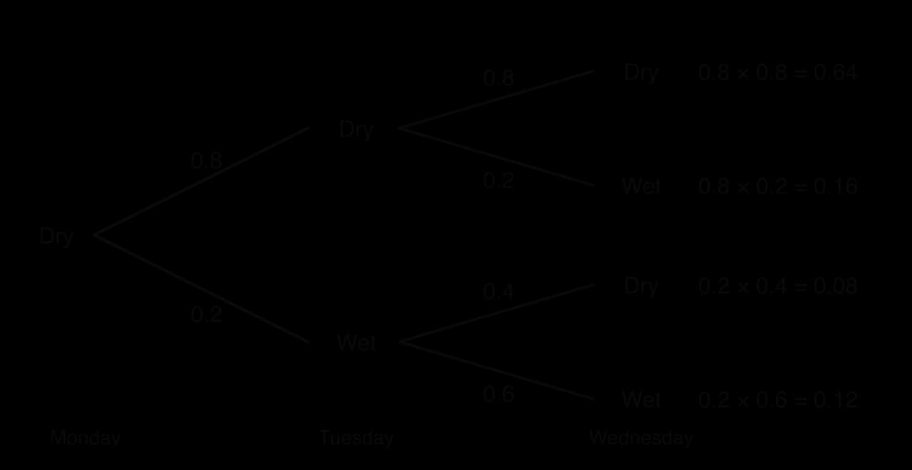
The probability of a dry Wednesday given a dry Monday is $0.8 \times 0.8 + 0.2 \times 0.4 = 0.72$, which is row 1 of $T$ multiplied by column 1 of $T$. The same reasoning applies to every entry, so $T^2$

In general, the entry in row $i$, column $j$ of $T^n$ is the probability of being in state $i$ exactly $n$ steps after being in state $j$

Counting the steps

The power is the number of transitions, not the number of days mentioned. From Monday to Wednesday there are two transitions (Monday → Tuesday → Wednesday), so the power is 2. From day 1 to day 30 there are 29 transitions. From "this week" to "in four weeks' time" with weekly steps there are 4.

Using the GDC

Matrix powers by hand are slow and error-prone beyond $T^2$, and the GDC does them directly.

1. Enter $T$ in the matrix editor (as matrix A, say) with the correct dimensions, column by column from the "from" states.

2. Enter $\boldsymbol{s}_0$ as a separate matrix with one column (matrix B).

3. On the home screen, compute $A^n \times B$, for example $A^{3}B$

On a TI-84 Plus CE the matrix editor is under 2nd x⁻¹ (MATRIX) → EDIT; on a Casio fx-CG50 it is in the Run-Matrix application. On any model, write down the matrix calculation and the resulting vector, not keystrokes.

State vectors of counts

When the state vector holds numbers, $T^n\boldsymbol{s}_0$ gives the expected numbers in each state after $n$ steps. The results need not be whole numbers, because they are averages over the random moves of every member. They are rounded only at the end, and only as far as the context requires.

Going back one step

Since $\boldsymbol{s}_n = T\boldsymbol{s}_{n-1}$, the previous state can be recovered with the inverse matrix whenever $T$ is non-singular: $\boldsymbol{s}_{n-1} = T^{-1}\boldsymbol{s}_n$

Yesterday was dry with probability 0.75. The inverse has negative entries, so it is not a transition matrix and cannot be read as "probabilities of moving backwards"; it only undoes the arithmetic. If going back produces a negative entry, the given vector could not have come from the chain in one step.

Long-term behaviour and the steady state

What happens to sₙ as n grows

Continuing the weather model from a dry day and from a wet day shows a clear pattern. Using the eigenvalues of $T$ (1 and 0.4, from subtopic 1.15), the probability of a dry day after $n$ steps is $\frac{2}{3} + \frac{1}{3}(0.4)^n$

The two sequences approach the same value, $\frac{2}{3}$, from opposite sides. After about a week, the weather on the starting day has almost no influence on the forecast. The gap from $\frac{2}{3}$ shrinks by a factor of 0.4 each day, which is the second eigenvalue of $T$

The steady state

The limit is a state vector that one more step leaves unchanged. If $\boldsymbol{s}_n$ settles to a vector $\boldsymbol{s}$, then taking the limit of both sides of $\boldsymbol{s}_{n+1} = T\boldsymbol{s}_n$

The steady state does not mean the system stops moving. Individual days still switch between dry and wet; what stays fixed is the proportion. In the bike-share scheme in its steady state, bikes still travel between stations every day, but the flows balance so that each station ends each day with the same expected number of bikes.

A long-term probability can also be read as the long-run proportion of steps the system spends in that state. Over a long period in the weather model, about two days in every three are dry.

There are three ways to find the steady state, each suited to a different form of answer. All three give the same result for a regular chain.

Method 1: a high power of T

For large $n$, every column of $T^n$ approaches the steady state. On the GDC,

The two columns are identical, and this is the sign that the power is high enough. The columns are identical because column $j$ of $T^n$ is $\boldsymbol{s}_n$ for a start in state $j$, and in the long run the start does not matter. Multiplying

The high-power method gives decimals. When exact values are needed, a decimal such as 0.667 is not the exact value $\frac{2}{3}$, and converting it to $\frac{667}{1000}$ does not make it exact either: the exact value comes from solving equations.

Method 2: solving Ts = s

To find the steady state exactly, write it as $\boldsymbol{s} = \begin{pmatrix} p \\ q \end{pmatrix}$ with $p + q = 1$

Both equations simplify to $0.2p = 0.4q$, that is $p = 2q$. The two equations always say the same thing, because adding them gives $p + q = p + q$

For an $n$-state chain, $T\boldsymbol{s} = \boldsymbol{s}$ gives $n$ equations, of which only $n - 1$ are independent. Any $n - 1$

The result confirms what the diagram suggested. The Harbour ends up with the largest share, 45%, although it started with only a third of the bikes, and the Park falls from half the bikes to 35%. A scheme operator could use it to plan how many bikes to move back to the Park each night.

A formula for two-state chains

Any two-state transition matrix can be written as

where $a$ is the probability of moving from state 1 to state 2 and $b$ the probability of moving from state 2 to state 1. In the steady state, the expected flow out of state 1 equals the flow into it: $a\,p = b\,(1 - p)$. Solving gives

For the weather model, $a = 0.2$ and $b = 0.4$, so $p = \frac{0.4}{0.6} = \frac{2}{3}$

Method 3: the eigenvector for the eigenvalue 1

The equation $T\boldsymbol{s} = \boldsymbol{s}$ is the eigenvector equation $T\boldsymbol{s} = \lambda\boldsymbol{s}$ of subtopic 1.15 with $\lambda = 1$. So the steady state is an eigenvector of $T$

Every transition matrix has 1 as an eigenvalue. Subtracting 1 from each diagonal entry of $T$ takes 1 away from exactly one entry in each column, so every column of $T - I$ sums to 0. The rows of $T - I$ then add up to a row of zeros, so they are linearly dependent and $\det(T - I) = 0$

An eigenvector can be multiplied by any non-zero number and remain an eigenvector, so the eigenvector itself is a whole family of vectors pointing the same way. The steady state is the one member whose entries sum to 1. An eigenvector with integer entries is convenient for exact work, because dividing each entry by the sum of the entries gives the exact steady state.

The eigenvector method links Markov chains to diagonalisation. Writing $T = PDP^{-1}$ gives $T^n = PD^nP^{-1}$

YouTube

Finding when a probability passes a threshold

Planning often needs the first step at which a probability reaches a given level. The GDC can list $\boldsymbol{s}_n$ for successive $n$, or a formula for $\boldsymbol{s}_n$ can be solved. Because $n$

The answer must be turned back into the context: six steps after Monday is Sunday, not "day 6". Counting the starting day as step 0 avoids an off-by-one error.

Regular Markov chains

Conditions for a unique steady state

The weather and bike-share chains settle to one steady state from any start. Not every chain behaves like this. Two examples show what can go wrong.

• A light that switches every second, on to off and off to on, has $T = \begin{pmatrix} 0 & 1 \\ 1 & 0 \end{pmatrix}$. The vector $\begin{pmatrix} 0.5 \\ 0.5 \end{pmatrix}$

The property that rules out both problems is that, after some fixed number of steps, every state can be reached from every state.

For a regular chain:

• there is exactly one steady state, and all its entries are positive;

• the columns of $T^n$ all approach that steady state as $n$ grows, so $T^n$ approaches a matrix with identical columns;

• $\boldsymbol{s}_n$

The second point is how the high-power method works, and the third is why the weather forecast for a day far ahead does not depend on today's weather. A transition matrix with no zero entries at all is regular with $k = 1$.

Regular chains and the convergence of Tⁿ

For a regular two-state chain, the second eigenvalue $1 - a - b$ lies strictly between $-1$ and 1, so its powers tend to 0 and only the steady-state part survives. For the switching light, $a = b = 1$ and the second eigenvalue is $-1$

A negative second eigenvalue, such as $-0.5$, still gives convergence, but $\boldsymbol{s}_n$ then overshoots the steady state on alternate steps, approaching it from above and below in turn. This happens when switching states is more likely than staying, as in Markov's chain of vowels and consonants.

Absorbing states

States that cannot be left

Some chains contain a state that, once entered, is never left: a game that has ended, a customer who has closed an account permanently, a machine that has been scrapped.

In the transition matrix, an absorbing state $j$ has a 1 on the leading diagonal in column $j$ and 0s in the rest of that column. In the transition diagram it has a loop labelled 1 and no arrows leaving it. A chain with an absorbing state that can be reached from every other state is not regular, because no power of $T$ can have a non-zero entry for a move out of the absorbing state.

A board game in which a player's next square depends only on the current square and the roll of a die, such as Snakes and Ladders, can be modelled as an absorbing chain. The squares are the states and the final square is the absorbing state. Powers of the transition matrix give the probability that the game has finished within a given number of turns.

Gambler's ruin

A classic absorbing chain is the gambler's ruin problem. A gambler with £2 bets £1 at a time, winning each bet with probability 0.4 and losing with probability 0.6, and stops on reaching £0 (ruin) or £4 (the target). The states are the amounts of money, £0 to £4, and £0 and £4 are absorbing.

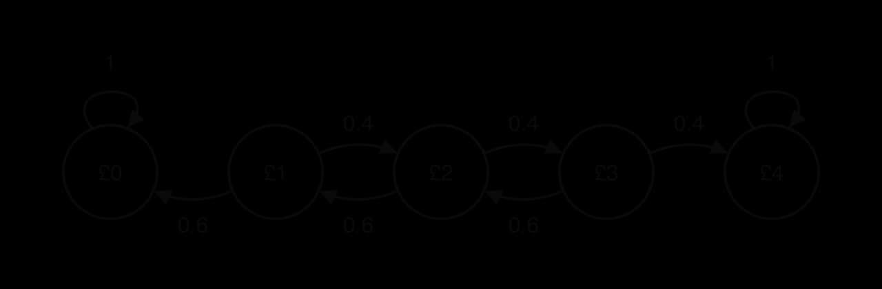
With the states in the order £0, £1, £2, £3, £4, the transition matrix and initial state vector are

The GDC gives $G^{100}\boldsymbol{s}_0 = \begin{pmatrix} 0.692 \\ 0 \\ 0 \\ 0 \\ 0.308 \end{pmatrix}$

Unlike a regular chain, this chain has a long-term state that depends on where it starts: from £3 the chance of reaching £4 rises to about 0.585. The equation $G\boldsymbol{s} = \boldsymbol{s}$ has many solutions, any mixture of "all at £0" and "all at £4", so there is no single steady state, and the columns of $G^n$ do not become identical.

Case study: Markov's vowels and consonants

Andrey Markov published his first paper on the chains named after him in 1906, to show that averages can settle down even when successive events are not independent. In 1913 he tested the idea on real data: he took the first 20,000 letters of Alexander Pushkin's novel in verse Eugene Onegin, classified each letter as a vowel (V) or a consonant (C), and counted the pairs of consecutive letters.

Source: counts from Markov (1913) as reported by O. Schwartz, IEEE Spectrum, 2019, and H. K. Strick, MacTutor History of Mathematics, St Andrews.

Building the chain

If letters were independent, the probability that a vowel follows a vowel would be the overall proportion of vowels, 0.432, and about $0.432^2 \times 20\,000 \approx 3730$ vowel–vowel pairs would be expected. Markov found 1,104, less than a third as many. The next letter clearly depends on the current one, so a two-state Markov chain with states V and C is a natural model.

The transition probabilities come from the pair counts. Of the roughly 8,640 vowels, 1,104 are followed by another vowel, and of the roughly 11,360 consonants, 3,827 are followed by another consonant:

The other two probabilities complete each column: $\mathrm{P}(\text{V} \to \text{C}) \approx 0.872$ and $\mathrm{P}(\text{C} \to \text{V}) \approx 0.663$. With the states in the order V, C,

The steady state and what it shows

Using the two-state formula with $a = \mathrm{P}(\text{V} \to \text{C}) = 0.8722\ldots$ and $b = \mathrm{P}(\text{C} \to \text{V}) = 0.6631\ldots$

The steady state of the chain is 43.2% vowels, the same proportion Markov counted. The agreement follows from how the chain was fitted. In any string of letters, the number of switches from a vowel to a consonant and the number from a consonant to a vowel can differ by at most one, because a run of vowels that starts must end (here each is about 7,535, half of the 15,069 mixed pairs). That is the flow-balance equation $a\,p = b\,(1 - p)$ of the steady state, written with counts. A chain fitted to a long sequence therefore has a steady state almost exactly equal to the observed proportions, and the model reproduces the text's long-run make-up while also describing how letters follow one another.

The second eigenvalue of $T$ is $1 - a - b = 0.128 + 0.337 - 1 = -0.535$. It is negative because changing state is more likely than staying: a vowel is usually followed by a consonant and a consonant usually by a vowel. Starting from a vowel, the probability that the second letter after it is a vowel is 0.595, then 0.345 for the third: the probabilities overshoot 0.432 on alternate steps while closing in on it, which is the pattern of a language that tends to alternate its sounds.

Limitations

The model uses only the previous letter. Real text depends on longer stretches: the chance of a vowel after two consonants differs from the chance after one, and Markov himself also counted triples of letters for this reason. The probabilities also belong to one Russian text; another language or another writer would give a different matrix. Four probabilities reproduce the long-run share of vowels accurately, but predictions of longer patterns, such as the chance of three consonants in a row, rest on the Markov property, which the text satisfies only roughly.

Exam focus

Markov chains appear on Paper 1 as short questions (2–8 marks) and on Paper 2 as longer questions (10–15 marks), often combined with eigenvalues and diagonalisation from subtopic 1.15. On Paper 3 they appear inside investigations that link graphs and Markov chains, such as a robot or an animal moving around a maze. The recurring tasks are:

• Complete or draw a transition diagram; write down the transition matrix (marks for the right size, entries between 0 and 1, columns summing to 1, then each column correct).

• Find a probability or an expected number after $n$ steps with $T^n\boldsymbol{s}_0$.

• Find the steady state or long-term probability: by a high power, by solving $T\boldsymbol{s} = \boldsymbol{s}$

What to write down: the transition matrix itself (labelled if helpful), the product used, such as $T^{5}\boldsymbol{s}_0$, with the resulting vector, and for a steady state either the high power used with its matrix, or the equations solved, or the eigenvector and its scaling. Markschemes award the method mark for "attempting to raise the transition matrix to a large power", and they condone omitting $\boldsymbol{s}_0$ when the correct column is read from $T^n$

The examiners' reports on Markov chain questions repeat a few points. Entries are often placed wrongly in the matrix, not only transposed but scrambled; labelling "from" and "to" first prevents this. Exact answers must be exact: a GDC decimal for a long-term probability earns partial credit at most when a fraction is asked for. Candidates who diagonalise a matrix when a GDC power would do tend to make more errors.

Interpretation parts carry a mark only when the direction of the move is clear. For the fitness app, "the probability of becoming Inactive" is not enough for the entry in row 3, column 1; the answer must say that it is the probability that a user who is Active one week is Inactive the next week.

Practice questions

1. Each school day, Ravi either walks (W) or takes the bus (B). If he walks one day, the probability that he walks the next day is 0.75. If he takes the bus one day, the probability that he walks the next day is 0.5. (a) Write down the transition matrix, with states in the order W, B. [2] (b) Ravi walks on Monday. Find the probability that he walks on Wednesday. [2] (c) Find the exact long-term proportion of days on which Ravi walks. [3]

2. Find the values of $x$, $y$ and $z$ in the transition matrix $\begin{pmatrix} 0.5 & x & 0.1 \\ 0.3 & 0.6 & y \\ z & 0.1 & 0.7 \end{pmatrix}$

Summary

• A Markov chain moves between states in steps, and the probability of the next state depends only on the current state (the Markov property).

• A transition diagram shows the states as circles and the moves as labelled arrows and loops; the probabilities leaving each state sum to 1.

• In the transition matrix, $T_{ij}$ is the probability of moving from state $j$ to state $i$: column = from, row = to, and each column sums to 1.

• A state vector holds the probability of, or the number in, each state; $\boldsymbol{s}_1 = T\boldsymbol{s}_0$

Self-check

• To do:

  I can draw a transition diagram from a description, with loops for staying in a state.

• To do:

  I can write a transition matrix with "from" along the top and "to" down the side, and check that each column sums to 1.

• To do:

  I can find missing entries of a transition matrix and interpret any entry, naming the direction of the move.

• To do:

  I can write an initial state vector of probabilities or of counts.

• To do:

  I can explain why one step of a chain is the multiplication $T\boldsymbol{s}$.

• To do:

  I can count the number of transitions between two named days or times correctly.

• To do:

  I can find a probability or expected number after $n$ steps with $T^n\boldsymbol{s}_0$