4.16 Confidence intervals

Learning objectives

• Explain why an interval estimate of a population mean is more informative than a single value.

• Find critical values of the standard normal distribution and of the t-distribution for a given confidence level.

• Calculate a confidence interval for the mean of a normal population when the population standard deviation is known, by hand and with the GDC.

• Calculate a confidence interval for the mean of a normal population when the population standard deviation is unknown, from raw data, a frequency table, summary statistics or $\sum x$ and $\sum x^2$.

• Interpret a confidence interval correctly in context, and explain what the confidence level means.

• Determine whether a claimed value of the mean is supported by a confidence interval, and relate this to a two-tailed hypothesis test.

• Find the least sample size that gives an interval of a required width, and find the confidence level of a given interval.

Introduction

A sample mean is the natural estimate of a population mean, but on its own it gives no idea of how far it might be from the truth. Two different samples from the same population give two different means, so any single value is almost certainly a little wrong. A confidence interval replaces the single value with a range of plausible values for the population mean, together with a measure of how reliable the method of producing that range is.

Confidence intervals are how measured quantities are reported throughout science, medicine and industry. A food producer checks that the mean mass of its packets is close to the label, a laboratory reports the mean concentration of a sample with its uncertainty, and a polling organisation gives a result "plus or minus" a margin. In each case the width of the interval shows how precise the estimate is, and the confidence level shows how often the method succeeds.

YouTube

From a point estimate to an interval estimate

Suppose a bottling plant wants to know the mean volume $\mu$ of all the bottles its machine fills. It cannot measure every bottle, so it takes a random sample of 25 and finds that the sample mean is $\bar{x} = 502.3$ ml. The value 502.3 is a point estimate of $\mu$: a single number calculated from the sample. The sample mean is an unbiased estimator of $\mu$, so on average it is right, but any one sample mean is almost certainly not exactly equal to $\mu$

How far $\bar{x}$ is likely to be from $\mu$ depends on how much sample means vary. Subtopic 4.15 showed that for a random sample of size $n$ from a normal population with mean $\mu$ and standard deviation $\sigma$, the sample mean has its own distribution:

The standard deviation of this sampling distribution, $\frac{\sigma}{\sqrt{n}}$, is the standard error of the mean. It measures the typical distance between a sample mean and the population mean. For the bottles, if $\sigma = 4$

An interval built around $\bar{x}$, wide enough to allow for this variation, is far more useful than $\bar{x}$ alone. It shows both the best estimate (the centre) and the precision of that estimate (the width).

The stated proportion is chosen before the interval is calculated. Common choices are 90%, 95% and 99%, and 95% is by far the most widely used.

The two ends of the interval have their own name, because they are often quoted separately (for example, "the mean is at least 500.7 ml with 95% confidence").

The standard normal distribution and critical values

Every normal distribution can be turned into one standard shape by subtracting its mean and dividing by its standard deviation. This standard shape supplies the numbers that set the width of an interval.

The normal distribution of subtopic 4.9 is symmetric about its mean, so the standard normal curve is symmetric about 0. For a confidence level of 95%, the middle 95% of the area under the curve is wanted, which leaves 2.5% in each tail. The value of $z$ with 97.5% of the area to its left is 1.960 (to 4 significant figures), so 95% of the area lies between −1.96 and 1.96.

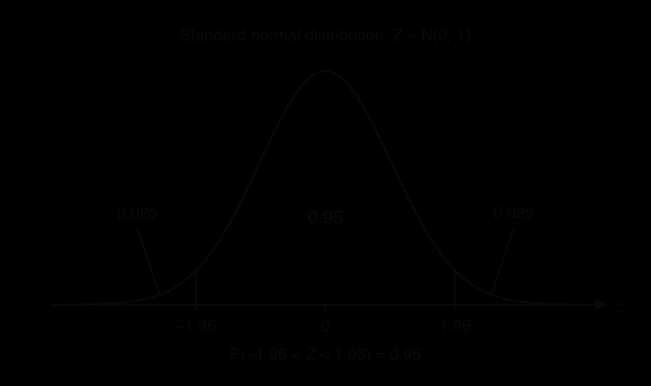
The number $z$ that cuts off the central area equal to the confidence level is the critical value for that level. It is found by an inverse normal calculation using the area to its left, which is $\frac{1 + c}{2}$ for a confidence level $c$ written as a decimal.

A higher confidence level needs a larger critical value, because more of the area has to be enclosed. On the GDC, the inverse normal function with area 0.975, mean 0 and standard deviation 1 gives 1.95996…; some models also accept a "centre" or "tail" setting that does the halving automatically.

Confidence intervals when σ is known

Deriving the interval

The interval comes straight from the distribution of $\bar{X}$. Standardising $\bar{X} \sim \mathrm{N}\left(\mu, \frac{\sigma^2}{n}\right)$

The last line says that the random interval from $\bar{X} - 1.96\frac{\sigma}{\sqrt{n}}$

The amount added to and subtracted from $\bar{x}$ is the part of the interval that reflects uncertainty, and it has its own name.

Calculating a z-interval

For the bottling plant, $\bar{x} = 502.3$ ml, $\sigma = 4$ ml and $n = 25$. The standard error is 0.8 ml, and the 95% margin of error is $1.95996 \times 0.8 = 1.568$

Using the GDC for a z-interval

The GDC's confidence interval functions do the whole calculation once the inputs are entered.

1. Open the interval functions: on a TI-84 Plus CE, STAT → TESTS → ZInterval; on a Casio fx-CG50, MENU → Statistics → INTR → Z → 1-S.

2. Choose the input type: Stats (summary values) or Data (a list of raw values, with a frequency list if the data are in a frequency table).

3. Enter $\sigma$, then either $\bar{x}$ and $n$ or the list, and the confidence level as a decimal (0.95).

4. Calculate. The GDC shows the lower and upper limits, $\bar{x}$

What to write down: the distribution used and its inputs, then the interval, for example "z-interval, $\sigma = 4$, $\bar{x} = 502.3$, $n = 25$, 95%: (500.7, 503.9)". A calculator command such as "ZInterval" on its own does not show the method.

What controls the width

The margin of error $z\frac{\sigma}{\sqrt{n}}$ has three ingredients, and each one changes the width in a predictable way. The table uses the bottling plant ($\bar{x} = 502.3$

• Confidence level. A higher level needs a larger $z$, so the interval widens. Being more confident of capturing $\mu$ costs precision: a 100% interval would have to include every possible value.

• Sample size. The margin is proportional to $\frac{1}{\sqrt{n}}$

The centre of a z-interval is always $\bar{x}$, and the interval is symmetric about it. This gives a quick check: the mean of the two confidence limits must equal the sample mean, and half their difference is the margin of error.

Interpreting a confidence interval

What 95% confidence means

The probability statement in the derivation is about the random interval, before the sample is taken. Once the data are in, $\bar{x}$ is a fixed number, the interval is fixed, and $\mu$ is also fixed (although unknown). The interval either contains $\mu$ or it does not; there is no longer anything random left to have a probability.

The 95% therefore describes the method, not one particular interval. If many random samples of the same size were taken and a 95% interval were calculated from each, about 95% of those intervals would contain $\mu$ and about 5% would miss it. Any single interval is one of these, and there is no way to tell from the data alone whether it is one of the successes.

A simulation shows this directly. Twenty random samples of size 10 were drawn by computer from a normal population with $\mu = 50$ and $\sigma = 10$, and a 95% z-interval was calculated from each. Every interval has the same width, $2 \times 1.96 \times \frac{10}{\sqrt{10}} = 12.4$

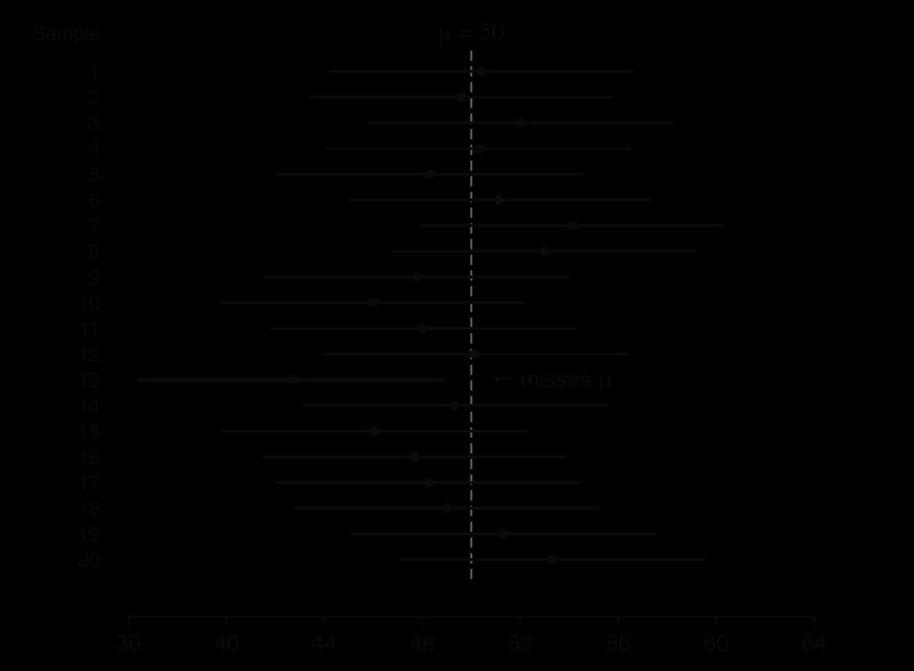
Across the twenty samples the intervals move while $\mu$ stays fixed. Interval 13 came from an unusually low sample mean (42.65) and misses $\mu$, even though it was calculated in exactly the same way as the others. With 20 intervals, about one miss is expected; in a different simulation there might be none, or two or three.

YouTube

What an interval does not say

Three further misreadings are common, and each comes from forgetting that the interval is about the mean of the population.

• An interval for the mean does not contain 95% of the individual values. Individual bottles vary with standard deviation 4 ml, so many bottles lie outside (500.7, 503.9); only the mean volume is estimated.

• An interval does not describe other samples. A second sample of 25 bottles would give a different interval; there is no guarantee that 95% of future sample means fall inside the first one.

• An interval allows only for random sampling variation. A biased sample, a badly calibrated measuring instrument or a population that is not normal can all make the interval wrong in ways that its width does not show. Michelson's 1879 measurements of the speed of light are a real example of an interval missing the true value for this reason.

Confidence intervals when σ is unknown

Why σ is usually unknown

The z-interval needs the population standard deviation $\sigma$. In practice $\sigma$ is rarely known: if the population had been studied well enough to know its spread exactly, its mean would usually be known too. Normally $\sigma$ is replaced by its estimate from the same sample, the unbiased estimate $s_{n-1}$, which the GDC labels $s_x$

Replacing $\sigma$ by $s_{n-1}$ adds a second source of variation. With $\sigma$ known, the standardised mean $\frac{\bar{X} - \mu}{\sigma/\sqrt{n}}$

The t-distribution

The distribution of this ratio was worked out at the start of the twentieth century and is now called the t-distribution (the story of its discovery is told in subtopic 4.11, Hypothesis testing).

The degrees of freedom measure how much information $s_{n-1}$ contains. A sample of $n$ values has $n - 1$ deviations from $\bar{x}$

Because more of the area lies in the tails, the critical value of a t-distribution for a given confidence level is larger than the matching $z$. The table gives 95% critical values (2.5% in each tail).

For a sample of 5 ($\nu = 4$) the multiplier is 2.776 instead of 1.960, an interval more than 40% wider; for a sample of 100 it is 1.984, only about 1% wider. The extra width allows for the uncertainty in estimating $\sigma$ from the same data.

The t-interval

The interval has exactly the same structure as the z-interval, with $s_{n-1}$ in place of $\sigma$ and a t critical value in place of $z$.

The choice between the two intervals depends only on whether the population standard deviation is known.

• $\sigma$ known (given in the question as the standard deviation of the population, the process or the machine): use the z-interval, whatever the sample size.

• $\sigma$ unknown (only sample data or a sample standard deviation available): use the t-interval with $s_{n-1}$ and $\nu = n - 1$

Calculating a t-interval from raw data

The GDC finds $\bar{x}$ and $s_{n-1}$ from a list and builds the interval in one step: on a TI-84 Plus CE, STAT → TESTS → TInterval; on a Casio fx-CG50, MENU → Statistics → INTR → t → 1-S. With Data input it needs only the list and the confidence level.

Calculating a t-interval from summary statistics

Questions often give only the sample mean and a sample standard deviation. The standard deviation must be checked: if it was calculated with divisor $n$ (written $s_n$, or described as "the standard deviation of the sample"), it has to be converted with the formula from subtopic 4.14 before it is used.

Calculating a t-interval from Σx and Σx²

When a sample is summarised by its size, the sum of the values and the sum of their squares, the two estimates come from formulas. The unbiased variance estimate in this form is

which is the sum of squared deviations from the mean, $\sum (x - \bar{x})^2$, written in a form that needs only the two sums. The values of $\bar{x}$, $s_{n-1}$

Data in a frequency table

When data are given in a frequency table, the values go in one GDC list and the frequencies in another, and the frequency list is named in the interval's Freq setting (or in one-variable statistics). The sample size is the total frequency, not the number of rows.

The lengths of 50 randomly chosen leaves from a species of tree, measured to the nearest centimetre, are shown in the frequency table.

Assumptions behind the intervals

Both intervals rest on the same assumptions, and an interval is only as good as they are.

• Random sample. The values must come from a random sample, so that $\bar{x}$ is unbiased and the values are independent. A convenience sample can give a narrow, precise-looking interval around the wrong value.

• Normal population. The distribution of $\bar{X}$ is exactly normal only when the population is normal. For a large sample from a non-normal population, the central limit theorem makes $\bar{X}$

A statement that "all conditions for a confidence interval have been met" refers to these three conditions.

Case study: Michelson's 1879 measurements of the speed of light

In June and July 1879, the physicist Albert Michelson measured the speed of light in air with a rotating-mirror apparatus at the United States Naval Academy. His 100 measurements were made in five experiments of 20 runs each, and they have become a standard dataset for teaching estimation. Each value is recorded in km/s with 299,000 subtracted, so a recorded 850 means 299,850 km/s.

Source: A. A. Michelson's 1879 measurements, as compiled by S. M. Stigler (1977), Annals of Statistics, and distributed as the R dataset morley/michelson (Rdatasets, accessed 2026).

Treating all 100 runs as one random sample from a normal population with unknown $\sigma$, a 95% t-interval with $\nu = 99$ is

that is, from 299,836.7 km/s to 299,868.1 km/s. Even a 99% interval, (831.6, 873.2), is only about 42 km/s wide, a very precise measurement for 1879.

On the same coded scale, the currently accepted value of the speed of light in air is 734.5. It lies about 102 km/s below the lower limit of the interval for all 100 runs, and below the interval for every one of the five experiments, as the chart of the six intervals shows.

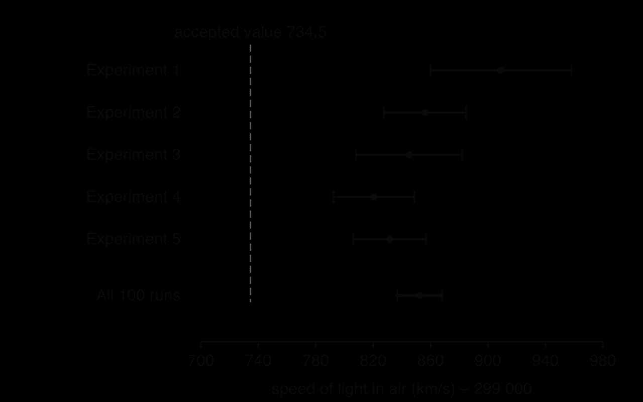
The miss is not one of the 5% of failures expected from random sampling. A 95% interval allows for random error, the scatter of individual runs around their own average. It cannot allow for systematic error, a bias that shifts every run in the same direction, such as a calibration fault in the measurement of distance or of the mirror's rotation rate. A systematic error moves the whole interval, and a larger sample only makes the wrongly placed interval narrower.

The five experiments give a second warning. Experiment 1's interval (859.9, 958.1) does not overlap experiment 4's (792.4, 848.6) at all, which suggests that the conditions changed between experiments, so the 100 runs are not really a single random sample from one population. The assumption of independent, identically distributed measurements behind the interval is therefore doubtful, and the interval for all 100 runs is narrower than the real uncertainty.

Using a confidence interval to judge a claim

Inside or outside the interval

A confidence interval gives the range of values of $\mu$ that are consistent with the data at the chosen level. Comparing a claimed value $\mu_0$ with the interval gives a quick judgement of the claim.

• If $\mu_0$ lies inside the interval, the data are consistent with the claim. The claim is plausible; it has not been proved, because many other values are plausible too.

• If $\mu_0$ lies outside the interval, the data give evidence against the claim, and the direction (above or below the interval) shows which way the true mean is likely to differ.

The conclusion must refer to the claim in its context: "the claimed mean of 250 g per tin lies outside the interval, so the manufacturer's claim appears to be incorrect (the mean mass is likely to be lower)".

The link with two-tailed tests

This comparison is equivalent to a two-tailed hypothesis test. Consider testing $\mathrm{H}_0\colon \mu = \mu_0$ against $\mathrm{H}_1\colon \mu \ne \mu_0$

A 95% interval matches a 5% test, a 90% interval a 10% test and a 99% interval a 1% test. The equivalence holds only for two-tailed tests that use the same distribution (z with z, t with t). The tests themselves, including one-tailed tests, are the subject of subtopic 4.18, Further hypothesis testing.

Choosing the sample size and the confidence level

The least sample size for a required width

Before collecting data, an investigator often wants an interval of a certain precision. When $\sigma$ is known, the width $w$ of a z-interval depends only on $z$, $\sigma$ and $n$, not on the data:

Requiring the width to be at most some value and solving the inequality for $n$ gives the least sample size. Because $n$ must be a whole number and a larger $n$ gives a narrower interval, the value found is always rounded up.

Finding the confidence level of a given interval

Sometimes the interval is given and the confidence level is unknown. When $\sigma$ is known, the margin of error gives the critical value, and a normal probability gives the level.

Exam focus

Confidence intervals appear in short Paper 1 questions (4–6 marks) and as parts of longer statistics questions in Papers 2 and 3, usually alongside unbiased estimates (subtopic 4.14), the distribution of $\bar{X}$ (subtopic 4.15) or hypothesis tests (subtopic 4.18). Typical parts are: find unbiased estimates of the mean and variance; find or calculate a confidence interval; comment on or explain whether a claim is supported; find the least value of $n$. The interval itself usually earns (M1) for an attempt with the right distribution and A1A1 (or A2) for the two limits. An interpretation earns an R1 mark only when it refers back to the claim in context.

The most frequent losses are using $s_n$ instead of $s_{n-1}$, using z when $\sigma$ is unknown (or t when it is known), giving $\bar{x} \pm$

Questions that give summary statistics test whether the right standard deviation is used. The phrases "the standard deviation of the sample", "$s_n$" or a GDC's $\sigma_x$ all mean the divisor $n$, and need converting; "an unbiased estimate of the variance" or "$s_{n-1}$

Practice questions

1. Write down the critical value $z$ used in a 98% z-interval. [1]

2. The scores on a reasoning test are normally distributed with standard deviation 15. A random sample of 36 students has mean score 104.2. Calculate a 90% confidence interval for the mean score of all students. [3]

3. The lengths, in cm, of seven randomly chosen fish of one species are 23.1, 24.6, 22.8, 25.0, 23.9, 24.2, 23.5. Lengths are normally distributed. Find a 99% confidence interval for the mean length of all fish of this species. [3]

4. For a random sample of 24 batteries, the lifetimes $x$ hours satisfy $\sum x = 868$ and $\sum x^2 = 31\,650$

Summary

• A confidence interval gives a range of plausible values for a population mean; its confidence level is the proportion of all samples for which the method captures $\mu$.

• With $\sigma$ known, the z-interval is $\bar{x} \pm z\frac{\sigma}{\sqrt{n}}$

Self-check

• To do:

  I can explain the difference between a point estimate and a confidence interval.

• To do:

  I can find the critical value $z$ for any confidence level using the area $\frac{1 + c}{2}$.

• To do:

  I can derive the z-interval from the distribution of $\bar{X}$