4.15 The central limit theorem · IB Maths AI | Augment Education
4.15 The central limit theorem
Use the fact that combinations of independent normal variables are normal, find the distribution of a sample mean and of a sum, and apply and state the central limit theorem for large samples from any population.
IB Mathematics: Applications and Interpretation
Part of 4 Statistics and probability
HL only
Key terms introduced here
Each is in the Maths AI glossary, with every other term in the subject.
The population, or the probability distribution, from which the observations in a sample are drawn; its mean μ and variance σ2 describe a single observation.
The standard deviation of the sampling distribution of the sample mean, nσ, where σ is the population standard deviation and n the sample size.
Notes on 4.15 The central limit theorem
32 min readLast reviewed
Learning objectives
State that a linear combination of independent normal random variables is normally distributed, and use it to find probabilities.
Find the mean, variance and standard error of the sample mean Xˉ of n independent observations.
UseXˉ∼N(μ,nσ2) to find probabilities about a sample mean when the population is normal, for any sample size.
State the central limit theorem in words, with its conditions.
Use the central limit theorem to find approximate probabilities for the mean or the sum of a large sample (n>30) from any population.
Justify whether a normal model for a sample mean or a sum is exact, approximate or not appropriate.
Explain why the sample size needed depends on the shape of the population, and why independence is required.
Introduction
A single measurement can be very unpredictable: one eruption of a geyser, one customer's spending, one wait for a bus. An average of many such measurements is far more predictable, and its behaviour follows a pattern that hardly depends on what the individual measurements look like. However skewed, lumpy or flat the population is, the mean of a large random sample has a distribution close to the bell-shaped normal curve, centred on the population mean, with a spread that shrinks as the sample grows.
This result, the central limit theorem, is the reason the normal distribution appears throughout statistics. It allows a manufacturer to judge a whole batch from the mean of a sample, a pollster to give a margin of error, and a scientist to attach an uncertainty to an average of repeated measurements. It is the foundation of the confidence intervals and hypothesis tests for a mean in subtopics 4.16 and 4.18.
YouTube
3Blue1Brown, “But what is the Central Limit Theorem?”: watch how the distribution of a sum of dice, starting from very different single-die distributions, settles into the same bell shape as more dice are added.
Linear combinations of independent normal variables
Subtopic 4.14 gives the mean and variance of any linear combination a1X1±a2X2±⋯±anXn
If X1,…,Xn are independent and normal, then a1X1±a2X2±⋯±anXn is normal.
Its mean and variance come from the rules in subtopic 4.14 for a linear combination of random variables: the means combine with the coefficients and signs, and the variances combine with squared coefficients and are always added. With the shape known as well, every probability for a total, a difference or a multiple can be found from the normal cdf on a GDC.
The result can be accepted without proof, and an informal argument makes it plausible. A normal variable can be thought of as the sum of very many small, independent random effects (heights depend on many genes and environmental factors; a measurement error collects many small disturbances). Adding two such variables just gives a larger collection of small independent effects, which is again normal.
When a combination has many terms, the method is the same; only the bookkeeping grows. Writing the combined variable in full before calculating keeps the number of terms right.
The distribution of the sample mean
A random sample of n observations X1,X2,…,Xn
The observations of a random sample have the same distribution as the parent population and do not influence one another. This pair of conditions has its own name.
The distribution of Xˉ over all possible samples of the same size has its own name.
Mean and variance of the sample mean
The sample mean is the linear combination Xˉ=n1X1+n1X2+⋯+n1Xn
E(Xˉ)Var(Xˉ)=n×n1μ=μ=n×(n1)2σ2=nσ2
The sample mean is centred on the population mean, and its variance is the population variance divided by the sample size. Its standard deviation, which measures how far a sample mean typically falls from μ, has a special name.
The square root in nσ has a practical consequence. To halve the standard error, the sample must be four times as large; to divide it by 10, a hundred times as large. Each extra observation improves precision, but by less and less.
When the parent population is normal
If the parent population is normal, Xˉ is a linear combination of independent normal variables, so it is exactly normal, whatever the sample size:
X∼N(μ,σ2)⟹Xˉ∼N(μ,nσ2)
The graph of a normal population with mean 50 and standard deviation 12, together with the distributions of the means of samples of 4 and of 16, shows both features. The centre never moves. The spread shrinks from 12 to 412=6
One item or the mean of a sample
A single observation and the mean of several observations have very different spreads. The single observation uses σ; the mean uses nσ
Finding the sample size needed
Because the standard error depends on n, a required level of precision fixes a minimum sample size. The method sets up an inequality in nσ
The central limit theorem
When the parent population is not normal, Xˉ is not exactly normal. The central limit theorem says that it becomes approximately normal as the sample size grows, whatever the shape of the parent.
Three facts about Xˉ are worth separating, because only one of them comes from the central limit theorem:
Fact about Xˉ
When it holds
Where it comes from
E(Xˉ)=μ
always
linear combination rules (subtopic 4.14)
Var(Xˉ)=nσ2
The mean and variance are exact for every sample size. The theorem adds only the shape, and the shape is what allows normal probabilities to be used.
Why averaging produces a bell shape
A sample mean is extreme only if most of the observations in the sample are extreme in the same direction. For one die, a score of 6 has probability 61; for the mean of two dice to be 6, both must show 6, probability 361; for the mean of ten dice to be 6, all ten must, probability about 1.7×10⁻⁸
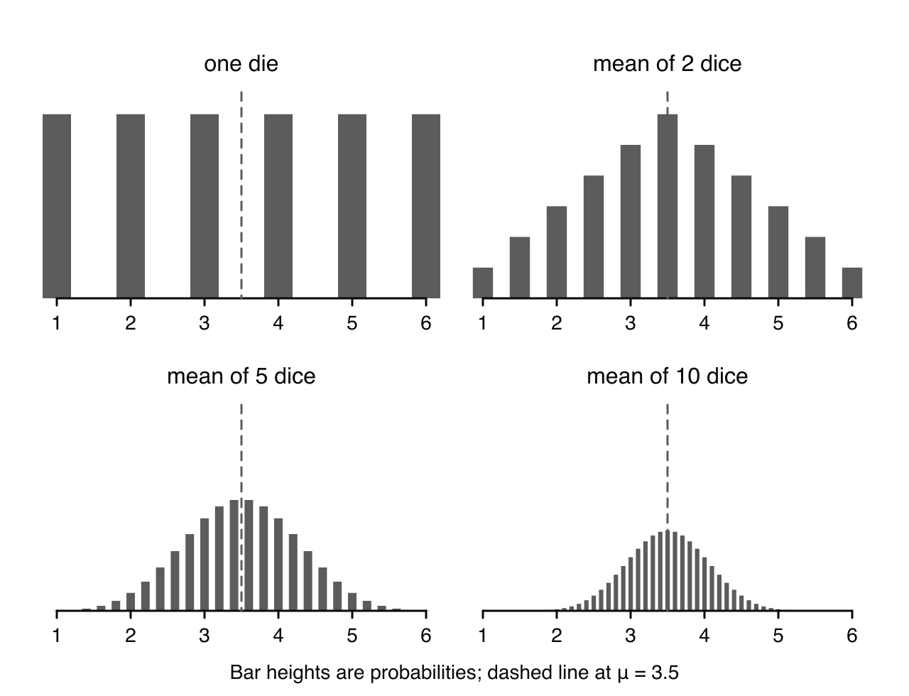
The mean of fair dice starts flat for one die, is triangular for two, and is already bell-shaped for five; every panel is centred on μ = 3.5 and the spread shrinks as n grows.
The exact distributions of the mean of 1, 2, 5 and 10 fair dice, drawn as bar charts, show how quickly the shape appears for a symmetric parent. One die has μ=3.5 and σ2=1235. For the mean of 10 dice, the variance is 1235÷10=0.292
The sample size needed for the theorem
The theorem describes a limit, so there is no single sample size at which Xˉ suddenly becomes normal. How large n must be depends on the parent population:
a normal parent needs no theorem: Xˉ is exactly normal for every n, even n=2;
a symmetric parent without extreme values (such as one die, or a uniform distribution) gives a nearly normal Xˉ
As a working rule, a sample of more than 30 is treated as large enough for the central limit theorem to apply. The rule is more than enough for a symmetric population and may fall short for a strongly skewed one.
YouTube
StatQuest with Josh Starmer, “The Central Limit Theorem, Clearly Explained!!!”: watch histograms of sample means taken from uniform and exponential populations turn into normal curves, and why this lets the normal distribution be used for means.
Stating the central limit theorem
A complete statement mentions four things: a large sample, the sample mean, that its distribution is approximately normal, and both parameters. An acceptable short form is:
For a sufficiently large random sample of size n from a population with mean μ and variance σ2, the sample mean Xˉ is approximately normally distributed with Xˉ∼N(μ,nσ2)
"Large" may be written as n>30 or "as n tends to infinity". Statements that leave out the sample mean ("the data become normal") or the variance are incomplete.
Case study: Old Faithful eruption durations
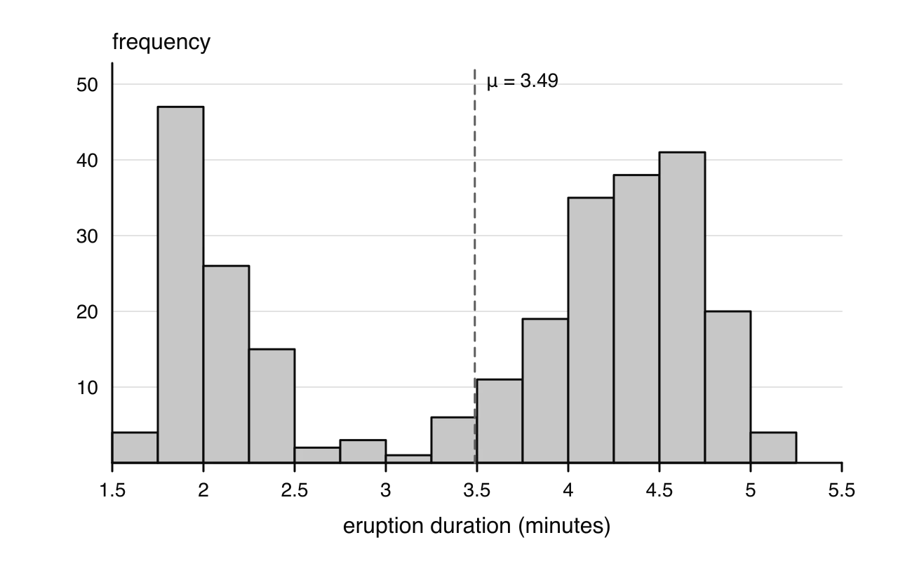
Old Faithful, a geyser in Yellowstone National Park, has eruptions of two kinds: short ones lasting about 2 minutes and long ones lasting about 4 to 5 minutes. A classic data set records 272 eruptions. Treating these 272 durations as the parent population gives μ=3.488 minutes and standard deviation σ=1.139 minutes (the unbiased estimate, if they are treated as a sample, is sn−1=1.141
The durations are bimodal, with about 36% of eruptions under 3 minutes and the rest over 3; the mean of 3.49 minutes sits at the lower edge of the long-eruption hump, and only about 6% of eruptions last within a quarter of a minute of it. Source: datasets::faithful (R), via Rdatasets, 2026.
The histogram of durations is very far from a normal curve. It has two separate humps with an almost empty gap between 2.5 and 3.25 minutes, and the mean, 3.49 minutes, lies at the lower edge of the second hump. Only 17 of the 272 eruptions (about 6%) last between 3.25 and 3.75 minutes, while a normal model with the same mean and standard deviation would put about 17% there, so a normal model for a single eruption would give misleading probabilities.
The central limit theorem gives a very different model for the mean duration of a random sample of 30 eruptions.
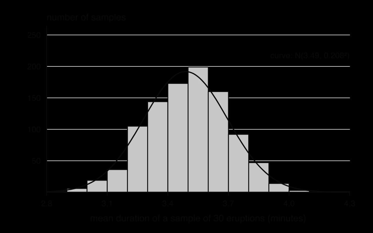
To check the prediction, 1000 random samples of 30 eruptions were drawn by computer (with replacement) from the 272 durations, and the mean of each sample was recorded. In this simulation the 1000 sample means had mean 3.50 minutes and standard deviation 0.199 minutes, close to the predicted 3.488 and 0.208.
Although single durations are bimodal, the means of samples of 30 form a single symmetric hump that the normal curve predicted by the central limit theorem fits closely. Simulation from datasets::faithful, 2026.
The histogram of the simulated sample means has a single peak at about 3.5 minutes, a duration that relatively few individual eruptions have, and the normal curve N(3.49, 0.208²) fits it well. The model allows probabilities about sample means to be calculated. For example, the probability that the mean of a random sample of 30 eruptions exceeds 3.8 minutes is about P(Xˉ>3.8)=0.0667 under Xˉ∼N(3.488,0.2082)
Two limitations matter. First, the simulation drew eruptions independently, but real consecutive eruptions are not independent: a short eruption tends to be followed by a long one, so 30 consecutive eruptions would not behave like a random sample. Second, the agreement is approximate; the theorem gives a good model for Xˉ at n=30 here because the durations, although bimodal, lie within a short range with no long tail, and a strongly skewed population would need larger samples.
Using the central limit theorem
The method mirrors the one for a normal parent, with one extra step: justify the normal model by the central limit theorem.
Identify μ and σ2 for one observation.
Check that n>30 and that the observations are independent (a random sample).
Write Xˉ≈N(μ,nσ2)
A symmetric parent such as a fair die needs far fewer observations than a skewed one, so an approximation based on 50 rolls is very close to the exact probability. The method is unchanged: the mean and variance of one roll, then the variance divided by n.
Deciding which model applies comes before any calculation. Two checks settle it, whether the parent population is normal and whether the sample is larger than 30, and they lead to an exact normal model, an approximate one, or none.
Sums of independent observations
Multiplying a sample mean by n gives the sample total, ∑Xi=nXˉ. A constant multiple of an approximately normal variable is approximately normal, so for large n the total is approximately normal too, with mean and variance from subtopic 4.14:
X1+X2+⋯+Xn≈N(nμ,nσ2)for large n
If the parent is normal, the total is exactly normal for any n. The events "Xˉ>k" and "∑Xi>nk
A load limit is a typical setting for a total. The total is approximately normal by the central limit theorem, and the number of items can then be varied to find how many are safe; since each n gives a different distribution, a table of probabilities on the GDC is the quickest way to search.
Independence and the limits of the theorem
Every result in the subtopic assumes that the observations are independent. The variance formula nσ2 and the central limit theorem both depend on it, because the cancelling of high and low values that narrows the distribution of Xˉ happens only when the observations do not move together.
Independence fails in recognisable ways:
observations close in time or space: temperatures on consecutive days, eruptions in a row, plants in the same patch of soil;
clusters: pupils from the same class, members of one family, passengers travelling as a group;
sampling without replacement from a small population: each item removed changes the population that remains.
When observations are positively related, the true variance of Xˉ is larger than nσ2, and probabilities based on the formula make the mean look more reliable than it is. Any use of these models should name the assumption: "the observations are independent", or "the sample is random".
A simulation of this kind does not prove the theorem, but it shows the two predictions that matter in practice: the centre of the sample means stays at μ, and their spread follows nσ
Exam focus
The central limit theorem is rarely the subject of a whole question, but the distribution of Xˉ underpins most questions on confidence intervals and tests for a mean (subtopics 4.16 and 4.18), and the normality of combinations is needed in almost every question on subtopic 4.14. It appears on Papers 1, 2 and 3. Typical demands:
state the distribution of Xˉ with both parameters (1–2 marks);
find the probability that a sample mean or a total lies in a range, for a normal parent or by the central limit theorem (3–5 marks);
explain or justify why a normal model can be used: "by the central limit theorem, since n is large", or "because the population is normal" (1–2 marks);
state the central limit theorem, or state an assumption (independence);
find a least sample size or a symmetric interval for a mean or a total, using the inverse normal.
Write the distribution, then the probability in correct notation; calculator syntax is not accepted. None of these results is in the formula booklet: Xˉ∼N(μ,nσ2)
The most frequent error in these questions is using the population standard deviation for a mean or a total. For a mean, the standard deviation is nσ; for a total of n
Practice questions
X∼N(20,32) and Y∼N(35,42) are independent. (a) FindP(X+Y>60)
Answers
(a) X+Y∼N(55,25); P(X+Y>60)=0.159
Summary
A linear combination of independent normal variables is normal; its mean and variance come from the rules of subtopic 4.14.
For n independent observations from a population with mean μ and variance σ2: E(Xˉ)=μ
Self-check
To do:
I can find probabilities for sums and differences of independent normal variables.
To do:
I can explain why the total of two dice is not normal but the total of two normal variables is.
To do:
I can derive E(Xˉ)=μ and Var(Xˉ)=nσ2
Questions on 4.15
30 exam-style questions on this subtopic, written in the style of the IB papers. The first has its markscheme open. Counted on
Question 1 · AI-009575 marks
The mass of honey in a jar filled by a machine at Ngata Apiaries, X grams, is normally distributed with mean 454 g and standard deviation 6.2 g.
A quality inspector selects a random sample of 12 jars and calculates their mean mass, Xˉ grams.
(a)
Find the probability that a single randomly selected jar contains less than 450 g of honey.
[1]1 mark
Markscheme (a)
0.259(0.259411…)A1
[1 mark]
(b)
Write down the distribution of Xˉ, stating its parameters.
[2]2 marks
Markscheme (b)
Xˉ∼N(454,126.22)
(c)
Find P(Xˉ<450).
[2]2 marks
Markscheme (c)
evidence of normal cdf with their distribution from part (b) (M1)
0.0127(0.0127118…)
Question 2 · AI-009587 marks
The passenger lift in the Torre Sabina office building displays the sign "Maximum load 1000 kg".
The masses of adults who use the lift are normally distributed with mean 76.5 kg and standard deviation 13.2 kg. Assume that the masses of the people in the lift are independent.
(a)
Twelve adults enter the lift. Let T be their total mass, in kg. Find the mean and the variance of T.
[2]2 marks
(b)
Find the probability that the total mass of the twelve adults exceeds the maximum load.
[2]2 marks
(c)
The building manager wants the probability that the total mass of the adults in the lift exceeds 1000 kg to be less than 1%. Find the greatest number of adults that should be allowed in the lift at one time.
Amara travels to work either by bus or by tram. Her journey time by bus, B minutes, follows the distribution N(34,4.52). Her journey time by tram, T minutes, follows the distribution N(31,2.82)
From the formula booklet
The entries of the mathematics: applications and interpretation formula booklet that 4.15 uses. Each opens in the explained booklet.
for a sample from a normal population, and the central limit theorem, with
n>30
taken as large enough. Probabilities are found with technology. The mean and variance of linear combinations are taught in subtopic 4.14, and the normal distribution itself in subtopic 4.9.
, but not its shape. In general the shape changes when random variables are combined: one die has a flat distribution, while the total of two dice is triangular. Normal variables are special, because combining them never changes the shape.
cm, independently of the top.
Find
the probability that a randomly chosen top fits a randomly chosen frame.
Show the solution
The top fits when the opening is longer than the top, that is when D=F−T>0.
E(D)=150.8−150.0=0.8,Var(D)=0.32+0.42=0.25
F and T are independent and normal, so D is normal: D∼N(0.8,0.25), with standard deviation 0.5.
Using the GDC's normal cdf with lower bound 0, mean 0.8 and standard deviation 0.5:
P(D>0)=0.945 (3 s.f.)
About 94.5% of tops fit. The average clearance of 0.8 cm is only 1.6 standard deviations of D, so about 1 pair in 18 does not fit.
g, all independent.
Find
the probability that a box weighs less than 2.6 kg.
Show the solution
Let B=J1+J2+⋯+J6+P, the mass of a box in grams.
E(B)=6(410)+150=2610,Var(B)=6(82)+122=528
Each jar contributes its own variance of 64; using 6J would wrongly give 36×64. Since B is a sum of independent normal variables, B∼N(2610,528).
P(B<2600)=0.332 (3 s.f.)
About one box in three weighs less than 2.6 kg.
is drawn from a population with mean
μ
and variance
σ2
. Before the sample is taken, its mean
Xˉ
is a random variable: a different sample would give a different value.
of
n
independent observations, each with mean
μ
and variance
σ2
. The rules from subtopic 4.14 give
is the population standard deviation and
n
the sample size.
For σ=12 and n=16, the standard error is 412=3.
one observation, N(50, 12²)
mean of 4, N(50, 6²)
mean of 16, N(50, 3²)
All three curves are centred on μ = 50; quadrupling the sample size halves the standard deviation, from 12 to 6 to 3, so sample means cluster ever more tightly around μ.
to
1612=3
, and the curves become taller because each still has total area 1.
. The second parameter of a normal distribution is the
variance
, which is
nσ2
. The standard deviation is
nσ
; this is the value entered as the standard deviation in the GDC's normal cdf.
, so its probabilities of extreme values are much smaller.
(3 s.f.), using mean 503 and standard deviation 6.
(b) The parent population is normal, so the mean of 10 packets is exactly normal:
Xˉ∼N(503,1062)=N(503,3.6)
The standard error is 106=1.897… g. Using the GDC's normal cdf with upper bound 500, mean 503 and standard deviation 106:
P(Xˉ<500)=0.0569 (3 s.f.)
Almost a third of single packets are under 500 g, but the mean of 10 packets falls below 500 g only about 5.7% of the time. Individual shortfalls are offset by packets that are over weight.
, uses the inverse normal for the boundary, and rounds
n
up
.
, where
Xˉ∼N(503,n36)
.
The value 500 must lie further below the mean than the point that cuts off the lowest 1% of a standard normal, z=−2.326…:
6/n500−503<−2.326…⟹n>32.326…×6=4.652…⟹n>21.6…
The least sample size is 22. Check with the GDC: for n=21, P(Xˉ<500)=0.0110, too large; for n=22, it is 0.00951, below 0.01. A table of P(Xˉ<500) for n=18,19,… on the GDC gives the same result without algebra.
". Examiners give a mark for using
Var(Xˉ)=nσ2
, and answers that use
σ
instead of
nσ
(treating the mean of the sample as one item) earn no further marks. An equivalent method uses the total
T=X1+⋯+Xn∼N(nμ,nσ2)
and is equally acceptable.
as
n
becomes large.
whenever the observations are independent
linear combination rules (subtopic 4.14)
Xˉ is normal
exactly, if the parent is normal; approximately, for large n, otherwise
normal combinations; the central limit theorem
. Values near the centre, on the other hand, can be made in very many ways, by combining high and low observations. As
n
grows, the probability piles up near
μ
and thins out symmetrically towards the extremes, which is the normal shape. The same mechanism drives the
Galton board
of subtopic 4.8, where each ball's final position is the sum of many independent left-or-right bounces.
, and the probability that the mean lies between 3 and 4 inclusive is already 0.687, compared with
31
for one die.
for
n
as small as 5 to 10;
a skewed parent, such as waiting times or incomes, needs larger samples, because the skewness of Xˉ fades only gradually as n increases;
a parent with very heavy tails or rare huge values may need samples of hundreds before the approximation is good.
and the theorem is not needed. Saying which of these applies is often worth a reasoning mark.
.
).
.
, "by the central limit theorem, since
n
is large".
Find the probability with the GDC's normal cdf, entering the standard deviation nσ.
Interpret the result in context, remembering that it is an approximation.
for negative waiting times, which are impossible.
(b) The sample is random and n=40>30, so by the central limit theorem
Xˉ≈N(12,4092),standard error 409=1.423…
Using the normal cdf with lower bound 14, mean 12 and standard deviation 409:
P(Xˉ>14)≈0.0799
The probability is about 0.0799. Because the parent is skewed, the true value may differ a little from this approximation.
. The rolls are independent and
n=50>30
, so by the central limit theorem
Xˉ≈N(3.5,5035/12)=N(3.5,0.05833…)
with standard error 0.05833…=0.2415…
P(3.3<Xˉ<3.7)≈0.592
The mean of 50 rolls is within 0.2 of 3.5 with probability about 0.592.
is too small for the central limit theorem; the mean of 8 incomes is still noticeably skewed.
(c) Approximately normal.n=60>30, so the central limit theorem applies (with some caution, because incomes are very skewed).
(d) Approximately normal. The theorem applies to discrete parents too; n=45>30 and the matches can be treated as independent.
" are the same event, so either form can be used; problems about a total amount (total sales, total time, total load) are usually clearer with the sum.
, so by the central limit theorem
Xˉ≈N(3.4,503.4)=N(3.4,0.068)
P(Xˉ>3.7)≈0.125
The probability is about 0.125. Equivalently, the total number of hires S over 50 days satisfies S≈N(170,170), and P(S>185)≈0.125. Here the exact answer is also available, because a sum of independent Poisson variables is Poisson: S∼Po(170) and P(S>185)=P(S≥186)=0.118. The approximation is good, but not perfect, because the normal model treats the discrete total as continuous.
. The sample of 40 is large (
n>30
) and the masses are independent, so by the central limit theorem
T≈N(58000,2704000)
, with standard deviation
2704000=1644
kg (4 s.f.).
(b) P(T>60000)≈0.112 (3 s.f.).
(c) For n cars, Tn≈N(1450n,2602n). The GDC's table of P(Tn>60000) for n=37,38,39,… gives
n
37
38
39
40
P(Tn>60000)
0.0000297
0.00112
0.0168
0.112
The probability is below 0.01 for n=38 but not for n=39, so the greatest number of cars is 38. The central limit theorem is used for 38 cars as well, since 38>30.
is only as valid as its conditions: a random sample of independent observations, and either a normal parent or a large enough
n
for the shape of the parent. Checking and stating these conditions is part of using the model correctly.
. With 100 stored means, the histogram is rough, but its single central peak is already clear.
?" (yes: approximately normal by the central limit theorem; no: no normal model). At the end of every route write
E(Xˉ)=μ
,
Var(Xˉ)=nσ2
, and the version for the total,
N(nμ,nσ2)
. Add one example of your own on each branch.
, the standard error
nσ
, the central limit theorem and the
n>30
convention must be learned, although the booklet's results for linear combinations (subtopic 4.14) give the mean and variance of
Xˉ
.
. [2]
Show the markscheme
(a) The mean is only 3.64.8=1.33 standard deviations above 0, and call lengths cannot be negative, so the distribution must be right-skewed (a normal model would give a substantial probability of negative lengths) R1
[1 mark]
(b) Xˉ≈N(4.8,503.62)A1A1
=N(4.8,0.2592)
by the central limit theorem, since n=50 is large (n>30) R1
Note: award the first A1 for the mean 4.8 and the second for the variance 0.2592 (accept 503.62); award A0 for a variance of 503.6
[3 marks]
(c) P(Xˉ>5.5)=0.0846(M1)A1
[2 marks]
(d) total T≈N(240,648)(A1)(A1)
P(T>260)=0.216A1
Note: accept P(Xˉ>5.2)=0.216.
[3 marks]
(e) inverse normal with area 0.05, mean 4.8, standard deviation 0.2592(M1)
k=3.96A1
[2 marks]
Total [11 marks]
independent observations, it is
nσ
; only a single observation uses
σ
.
. When it asks you to
justify
a normal model, say which reason applies: "the population is normal" (exact, any
n
) or "by the central limit theorem, as
n>30
" (approximate). When it asks for assumptions, state that the observations are
independent
.
. [3] (b)
Find
P(2X>Y+10)
. [4]
Exam scores are normally distributed with mean 72 and standard deviation 15. A random sample of 9 scores is taken. (a) Write down the distribution of the sample mean Xˉ. [2] (b) FindP(70<Xˉ<75). [2]
A measuring instrument gives readings that are normally distributed about the true value with standard deviation 2.4 units. Find the least number of independent readings needed so that the probability that their mean is within 0.5 units of the true value is at least 0.95. [4]
Weekly spending by customers of an online shop has mean $280 and standard deviation $190, and is strongly skewed. Find, approximately, the probability that the mean spending of a random sample of 60 customers exceeds $300. Justify the method. [4]
Items on a conveyor belt have masses with mean 1.2 kg and standard deviation 0.5 kg. A box holds 36 items chosen at random. Find, approximately, the probability that the total mass of the items in a box exceeds 45 kg. [4]
The number of emails a worker receives in an hour has a Poisson distribution with mean 3.6. Use the central limit theorem to find, approximately, the probability that the mean number per hour over 40 independent hours exceeds 4. [4]
A random number generator produces digits 0 to 9, each with probability 0.1, so that μ=4.5 and σ2=8.25. Find, approximately, the probability that the mean of 100 digits is less than 4.2. [3]
A clock chimes 49 times. The time intervals between successive chimes are independent, with mean 1.8 seconds and variance 0.05 seconds². (a) Find the mean and variance of the total time from the first chime to the last. [3] (b) Explain why a normal distribution can be used for the total time. [2] (c) Find an interval, symmetric about the mean, that contains the total time with probability 0.9. [3]
Explain the difference between the statement "the masses of 100 randomly chosen apples are normally distributed" and the central limit theorem applied to the same sample. [2]
. (b)
D=2X−Y−10∼N(−5,4×9+16)=N(−5,52)
;
P(D>0)=0.244
.
(a) Xˉ∼N(72,9152)=N(72,25). (b) 0.381.
Need 2.4/n0.5≥1.95996…, so n≥9.408, n≥88.5: 89 readings.
n=60>30, random sample, so by the central limit theorem Xˉ≈N(280,601902), standard error 24.53; P(Xˉ>300)≈0.207.
T≈N(43.2,36×0.25)=N(43.2,9) by the central limit theorem (n=36>30); P(T>45)≈0.274.
Xˉ≈N(3.6,403.6)=N(3.6,0.09); P(Xˉ>4)≈0.0912.
Xˉ≈N(4.5,0.0825); P(Xˉ<4.2)≈0.148.
(a) 48 intervals: mean 48×1.8=86.4 s, variance 48×0.05=2.4 s². (b) The total is a sum of 48 independent intervals, n=48>30, so the central limit theorem applies. (c) Inverse normal for N(86.4,2.4) with 5% in each tail: 83.9 s to 88.9 s (3 s.f.).
The first is a claim about the population of masses (one apple at a time); the central limit theorem is a claim about the sample mean of 100 masses, which is approximately normal even if single masses are not.
and
Var(Xˉ)=nσ2
, always.
The standard error of the mean is nσ; quadrupling n halves it.
If X∼N(μ,σ2), then Xˉ∼N(μ,nσ2) exactly, for every n.
Central limit theorem: for a large random sample from any population with finite variance, Xˉ is approximately N(μ,nσ2); n>30 counts as large.
How large n must be depends on the parent: small for symmetric populations, larger for skewed or heavy-tailed ones.
The total of n independent observations is approximately N(nμ,nσ2) for large n (exactly, for a normal parent).
The theorem is about the sample mean or total, not the data; it needs independent observations.
Write the distribution with both parameters (variance second) before any probability, and justify it by "normal parent" or "central limit theorem, n>30".
from the rules for linear combinations.
To do:
I can find the standard error nσ and explain what happens to it when n is multiplied by 4.
To do:
I can write Xˉ∼N(μ,nσ2) with the variance as the second parameter.
To do:
I can contrast the probability for one item with the probability for the mean of a sample.
To do:
I can find the least sample size for a required probability, rounding up.
To do:
I can state the central limit theorem with all four elements.
To do:
I can decide whether Xˉ is exactly normal, approximately normal or not justified as normal, and say why.
To do:
I can explain why the sample size needed depends on the shape of the parent population.
To do:
I can use ∑Xi≈N(nμ,nσ2) for a total, counting the number of terms correctly.
To do:
I can state independence as an assumption and give situations where it fails.
To do:
I can explain that the central limit theorem is about the sample mean, not about the data.
A1A1
(Xˉ∼N(454,3.20333…))
Note: Award A1 for normal with mean 454, A1 for variance 126.22 (or 3.20). Accept standard deviation 126.2=1.78979… if clearly labelled as the standard deviation.
[2 marks]
A1
[2 marks]
. All journey times are independent.
(a)
Find E(B−T) and Var(B−T).
[2]2 marks
(b)
On a randomly chosen day, find the probability that a bus journey would be quicker than a tram journey.
[2]2 marks
(c)
In one week Amara travels by tram on each of her 5 working days. Find the probability that her total travel time for these five journeys is more than 160 minutes.
 YouTube
 YouTube