A4.3 Machine learning approaches

Learning objectives

• Explain how linear regression uses the slope, the intercept and r² to predict continuous outcomes. (HL only)

• Explain how k-nearest neighbours and decision trees classify new data from labelled examples. (HL only)

• Explain the role of hyperparameter tuning, using accuracy, precision, recall and F1 score, and the ideas of overfitting and underfitting. (HL only)

• Describe how k-means clustering groups data by the similarity of its features. (HL only)

• Describe how association rules uncover relations in large data sets, and interpret support, confidence and lift. (HL only)

• Describe how an agent learns by interacting with its environment, including cumulative reward and the exploration–exploitation trade-off. (HL only)

• Describe how genetic algorithms solve optimisation problems such as the travelling salesperson problem. (HL only)

• Outline the structure and function of artificial neural networks, and sketch a perceptron and a multi-layer perceptron. (HL only)

• Describe how convolutional neural networks learn spatial hierarchies of features in images. (HL only)

• Explain why model selection and comparison matter in machine learning. (HL only)

Introduction

Machine learning (ML) covers many different techniques. Predicting a house price, flagging a medical scan, grouping a shop's customers, choosing a game move and planning delivery routes are different problems, and each suits a different family of algorithms. Choosing well needs an understanding of how each approach works: what it learns, what it assumes about the data, what it costs to run and how it fails. Honest measurement of performance on unseen data, and careful tuning, apply to all of them.

Linear regression

Many questions ask for a number rather than a category: how long a delivery will take, how much electricity a building will use tomorrow, what a second-hand car will sell for. These are regression tasks, a form of supervised learning in which each training example has a known numerical answer. The simplest regression model assumes that the answer changes at a steady rate as one input changes, so the relationship can be drawn as a straight line.

Independent and dependent variables

The input that is known, or that can be set, is the independent variable; the output being predicted is the dependent variable, because its value is assumed to depend on the input. In a model that predicts delivery time from distance, distance is independent and time is dependent.

The dependent variable is plotted on the vertical axis ($y$) and the independent variable on the horizontal axis ($x$). In machine learning terms, the independent variables are the features and the dependent variable is the label.

The regression equation: slope and intercept

A straight line is fixed by two numbers:

Here $\hat{y}$ ("y-hat") is the predicted value of the dependent variable, $x$ is the independent variable, $b_1$ is the slope and $b_0$

A slope of 3 in a model of delivery time (minutes) against distance (km) means that each extra kilometre adds 3 minutes to the predicted time. Its sign gives the direction of the relationship and its size the strength of the effect in the units of the problem, so a slope is always interpreted with its units.

The intercept is where the line crosses the vertical axis. In the delivery model an intercept of 10 minutes has a real meaning: the fixed time to prepare and load an order. Often, though, $x = 0$ is far outside the data (a house with a floor area of zero), and the intercept is then only a mathematical anchor for the line, not a usable prediction.

Fitting the line: residuals and least squares

Real data never lies exactly on a line. For each training example, the difference between the actual value and the predicted value is a residual, and a good line makes the residuals small overall.

Positive residuals (points above the line) and negative residuals (points below it) would cancel out if they were simply added, so the standard method squares each residual first and finds the line that makes the total as small as possible. Squaring also punishes large errors more than small ones: one residual of 4 contributes 16, the same as four residuals of 2.

A hypothetical bakery records the distance and time of six deliveries and fits a line by least squares. The scatter graph of the data shows the six points, the fitted line $\hat{y} = 10 + 3x$, and the residual of each point.

The least-squares formulas use the means $\bar{x}$ and $\bar{y}$ of the two variables. Computing them by hand is optional detail. The slope measures how $x$ and $y$ vary together relative to how much $x$

Goodness of fit: r² and r

A line can be fitted to any data, even data with no pattern, so a measure of fit is also needed. The coefficient of determination, written $r^2$, compares the errors of the line with the errors of the simplest possible model, which always predicts the mean $\bar{y}$.

$SS_{\text{tot}}$ is the total variation of $y$ around its mean, and $SS_{\text{res}}$ is the variation the line fails to explain. If the line predicts every point exactly, $SS_{\text{res}} = 0$

For the bakery, $SS_{\text{tot}} = 205.5$ (the sum of the squared values of $y - \bar{y}$) and $SS_{\text{res}} = 2^2 + 4^2 + 2^2 + 2^2 + 4^2 + 2^2 = 48$

A related measure is the correlation coefficient $r$. It describes the strength and direction of a straight-line relationship between two variables, from −1 (a perfect downward line) through 0 (no straight-line relationship) to +1 (a perfect upward line). For a model with one independent variable, $r^2$ is exactly the square of $r$, with the sign of $r$ matching the sign of the slope.

For the bakery data $r = +\sqrt{0.766} = 0.875$, a strong positive relationship. The correlation coefficient describes how closely two variables move together and in which direction; $r^2$

YouTube

The StatQuest video builds the same picture as the bakery example: the residuals around the mean, the smaller residuals around the fitted line, and R² as the fraction of variation removed by the line. A high r² still says nothing about cause. Ice-cream sales and drowning incidents are strongly correlated across the months of a year because both rise in hot weather; neither causes the other. A regression model finds an association in its data, and deciding whether changing $x$ would change $y$ needs a controlled experiment or knowledge of the mechanism.

Making predictions: interpolation and extrapolation

To predict, the new value of the independent variable is substituted into the equation, as for the 4.5 km delivery. A prediction inside the range of the training data is an interpolation and is usually trustworthy if the fit is good. A prediction outside that range is an extrapolation, which assumes that the straight-line pattern continues where no data was seen.

The bakery model predicts $10 + 3 \times 30 = 100$ minutes for a 30 km delivery. The training data stopped at 6 km, and over 30 km a van would probably use a faster road, so the true time could be far shorter. Extrapolation is risky for every kind of model, because no training example shows how the system behaves there.

Multiple regression

Multiple regression extends the idea to several independent variables, each with its own slope, so the model becomes a flat surface in more dimensions instead of a line. A house-price model might use floor area, number of bedrooms and distance from the city centre together, and each slope is then read as the effect of its variable while the others are held fixed.

Classification: k-nearest neighbours and decision trees

Classification predicts a category instead of a number: spam or not spam, which species a flower belongs to, which illness a set of symptoms suggests. The model learns from training data in which every example carries its correct class label, then assigns a label to each new example. k-nearest neighbours does this by comparing a new case directly with stored examples; a decision tree learns a set of questions that lead to an answer.

How k-nearest neighbours classifies

The idea behind k-nearest neighbours (k-NN) is that similar things tend to belong to the same class. Each example is a point in a space with one dimension per feature. To classify a new point, the algorithm finds the $k$ training points closest to it and takes a vote among their classes.

k-NN has no real training phase. It stores the labelled examples and does all of its work when a prediction is requested, so it is called a lazy learner: "training" is instant but prediction is slow, because every new point is compared with every stored point.

The k-NN algorithm in steps:

1. Choose $k$, the number of neighbours, and a distance measure.

2. Calculate the distance from the new point to every training point.

3. Sort the training points by distance and take the $k$ nearest.

4. Assign the class held by most of those $k$ neighbours (for regression, the mean of their values).

Measuring distance

The usual distance metric is Euclidean distance, the straight-line distance between two points, found with Pythagoras' theorem extended to any number of features:

An alternative is Manhattan distance, named after the street grid of Manhattan, where a taxi travels along the blocks rather than diagonally. It adds the absolute differences instead of squaring them, so one very large difference counts for less than in the Euclidean distance.

Distances only make sense if the features are on comparable scales. If one feature is income in dollars (tens of thousands) and another is age in years (tens), the income differences swamp everything else and age has almost no effect. k-NN is therefore almost always run after feature scaling, which puts every feature on a similar range.

The vote

Each of the $k$ nearest neighbours casts one vote for its own class, and the class with the most votes is the prediction. A variant, weighted voting, gives closer neighbours more say, for example by weighting each vote by one divided by its distance.

For a problem with two classes, $k$ is normally odd so that the vote cannot be tied. With three or more classes, ties are still possible and need a rule, such as taking the class of the single nearest neighbour.

Worked data: Fisher's Iris flowers

The Iris data set, published by the statistician Ronald Fisher in 1936, records four measurements of 150 iris flowers, 50 from each of three species (setosa, versicolor and virginica), and is a standard first data set for classification. The k-NN plot uses eight real flowers from it, four versicolor and four virginica, plotted by petal length and petal width, and a ninth flower to be classified: petal length 4.9 cm, petal width 1.5 cm.

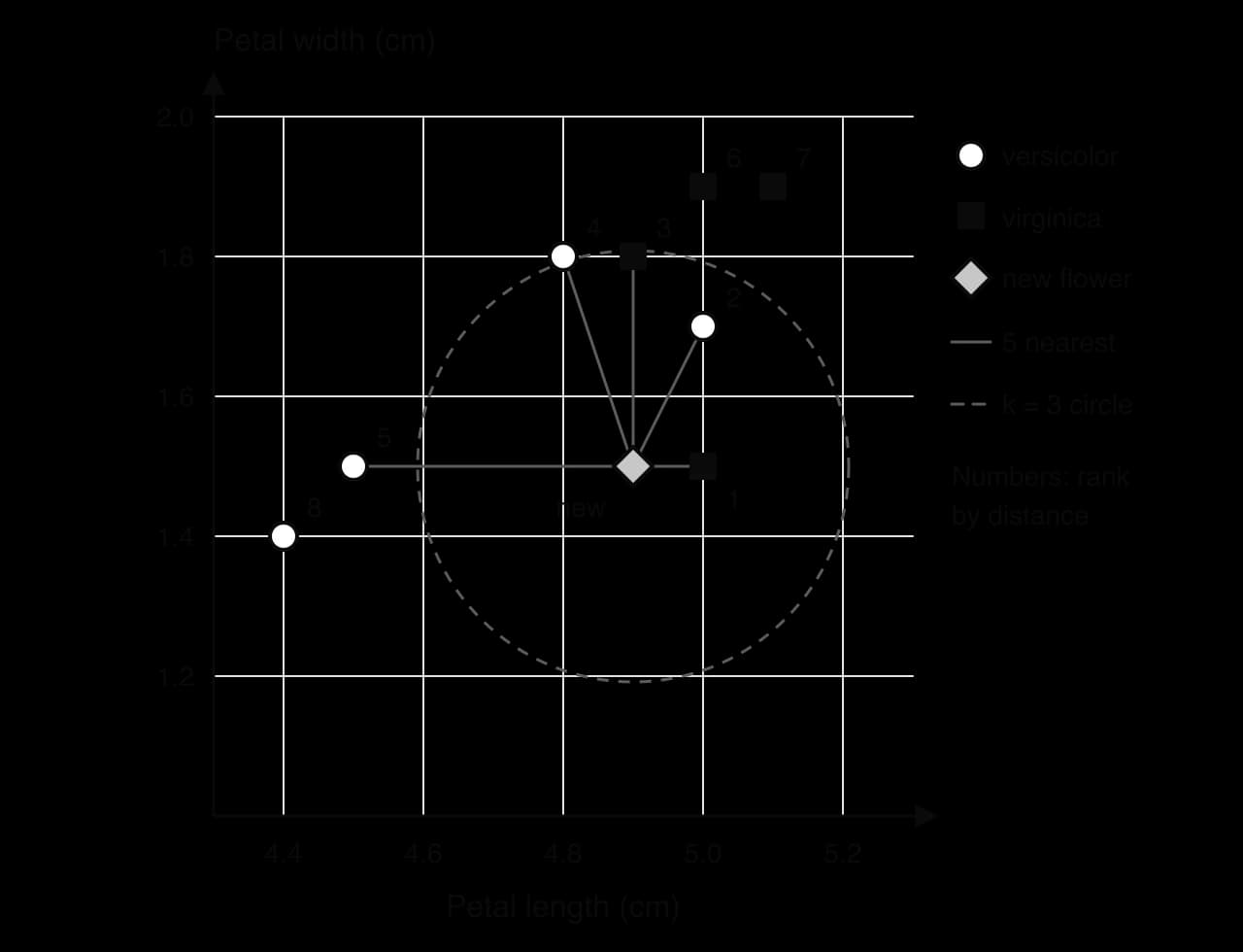
Source: Fisher's Iris data set (1936), flowers 52, 66, 71, 78 (versicolor) and 102, 120, 124, 147 (virginica), UCI Machine Learning Repository.

The distance table ranks the eight training flowers by their distance from the new flower. Both metrics give the same five nearest neighbours, although Manhattan distance produces ties.

The new flower is in fact flower 73 of the data set, a versicolor. With $k = 1$ or $k = 3$ the model is wrong, with $k = 5$ it is right, and with $k = 7$

Choosing k

The value of $k$ controls how smooth the model's decisions are. With $k = 1$, each training point alone sets the class of the space immediately around it, so a single mislabelled or unusual flower changes predictions near it and the model follows noise. With a very large $k$, the vote covers so much of the data that local detail disappears; when $k$ equals the size of the data set, every new point is given the most common class. Small $k$ therefore tends to overfit and large $k$

Strengths and limitations of k-NN

k-NN is simple to understand and explain ("these five similar cases were mostly versicolor"), needs no training time, and adapts at once when new labelled examples are added. Its costs come at prediction time. Classifying one point against $n$ stored points with $d$ features takes about $n \times d$ operations, which is $O(n)$ in Big O notation for a fixed number of features, and the whole training set must be kept in memory. With many features it also suffers from the curse of dimensionality: in high-dimensional space, points tend to be roughly equally far from one another, so "nearest" stops meaning "similar".

Collaborative filtering: k-NN in recommendation systems

A recommendation system predicts which products a person will like. One approach, collaborative filtering, uses the ratings of many users rather than any description of the products. In its neighbourhood form it is k-NN applied to people: each user is a point whose features are their ratings, the nearest neighbours are the users with the most similar tastes, and items those neighbours rated highly but the user has not seen are recommended.

A hypothetical streaming service holds these ratings (1 to 5) for four films. Ana has not yet seen film 4.

Over films 1–3, Ana's Euclidean distance is 1.00 from Dev ($\sqrt{0 + 1 + 0}$), 1.73 from Ben ($\sqrt{1 + 1 + 1}$

Because it needs no knowledge of the items, collaborative filtering works for films, songs and products alike. It has two well-known weaknesses. A new user or new item with no ratings cannot be placed among neighbours (the cold-start problem), and most users rate only a tiny fraction of items, so the ratings table is mostly empty, which makes distances unreliable.

Decision trees

A decision tree classifies an example by asking a sequence of questions about its features. It has the shape of an upside-down tree: the first question is at the root node, each internal node tests one feature, each branch is one possible answer, and each leaf node gives a class. To classify a new case, the algorithm starts at the root and follows the branch that matches the case's answer at each node until it reaches a leaf.

A hypothetical clinic has records of ten patients, with three symptoms and whether a test later confirmed flu. The tree learned from these records is shown in the diagram of the flu decision tree.

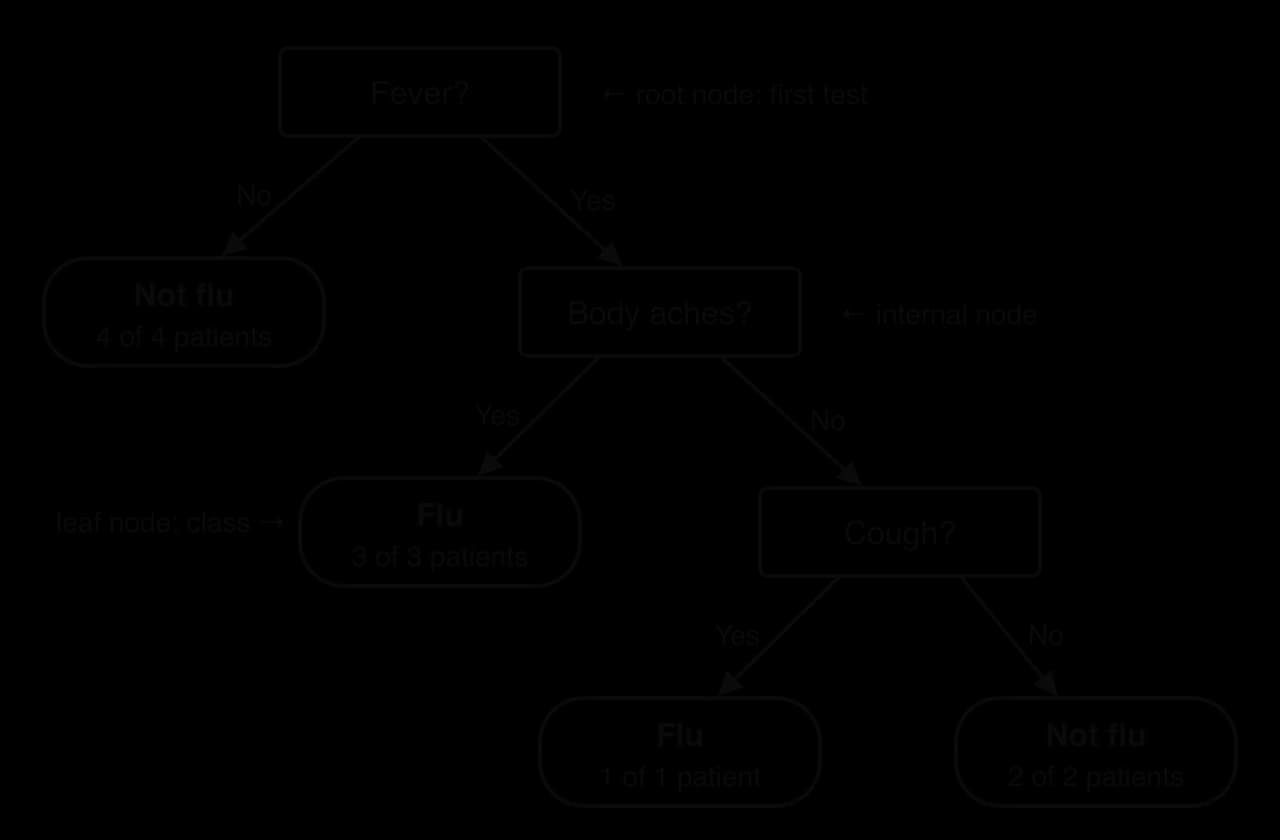
Every path in the tree reads as an if–then rule ("if the patient has a fever and body aches, predict flu"), which makes decision trees easy to check. A new patient with a fever, no body aches and a cough follows Fever = Yes, Body aches = No, Cough = Yes and is classified as flu. Real diagnostic trees support a clinician's judgement rather than replace it, and they use many more features, including numerical ones such as temperature, split with a threshold ("temperature > 38 °C?").

Building a tree: splitting criteria

A tree is built from the top down. At the root, the algorithm considers every feature it could split on and chooses the one that best separates the classes; it then repeats the process inside each branch with the training examples that reached it. A branch stops growing when all its examples share one class (the node is pure), when no features are left, or when a limit such as a maximum depth is reached. The measure used to compare candidate splits is the splitting criterion.

The most common criterion is Gini impurity. For a node in which a fraction $p_i$ of the examples belongs to class $i$:

A pure node has $G = 0$. For two classes the worst case is a 50/50 mix, $G = 1 - 0.5^2 - 0.5^2 = 0.5$

A second criterion, information gain, comes from information theory. It measures disorder with entropy, $H = -\sum_i p_i \log_2 p_i$

Pruning and the risk of overfitting

A tree that keeps splitting until every leaf is pure fits its training data exactly, noise included. The Cough? node in the flu tree rests on three patients and a leaf on one, so a single unusual patient could have produced it. Such a tree scores perfectly on its own training data but predicts poorly for new patients. Pruning controls this, either by stopping growth early (a maximum depth, or a minimum number of examples per leaf) or by growing the full tree and then removing branches that do not improve accuracy on separate validation data.

Pruning the flu tree at depth 2 would replace the Cough? node with a single leaf, "Not flu" (two of the three patients there), giving a simpler rule set that misclassifies one training patient but is less likely to reflect chance. Trees are also sensitive to small changes in the data: removing a few records can change the root split and so the whole tree. Ensembles such as random forests, which average many trees grown on different samples of the data, reduce this instability at the cost of the single tree's readability.

YouTube

The StatQuest video builds its tree with the same weighted Gini comparison as the flu example, and shows how a numerical feature is split by testing candidate thresholds.

Evaluating classifiers and tuning hyperparameters

A model is only useful if it makes good predictions on data it has never seen. Measuring that needs metrics that describe the kinds of mistake a model makes, and a careful procedure for choosing settings such as $k$ or a tree's depth without fitting the model to the very data used to judge it.

The confusion matrix

For a classifier with two classes, one class is called positive (usually the one being searched for: the disease, the spam, the fraud) and the other negative. Every prediction then falls into one of four outcomes, and counting them on test data gives a confusion matrix.

The four cells of a two-class confusion matrix have standard names. The first word says whether the prediction was right (true) or wrong (false); the second says what the model predicted (positive or negative).

A true positive is a sick patient whom the test flags as sick. Its mirror image is the healthy patient whom the test correctly clears.

The two kinds of error have different costs, so they are counted separately: a false positive is a false alarm and a false negative is a miss.

In statistics a false positive is called a type I error and a false negative a type II error.

A hypothetical screening test is applied to 1,000 people, 50 of whom have the condition. It correctly flags 40 of them and misses 10; of the 950 healthy people it wrongly flags 90 and correctly clears 860. The diagram of the confusion matrix shows these counts and which cells each metric uses.

Accuracy, precision, recall and F1 score

Accuracy is the fraction of all predictions that are correct. It is the most familiar measure, but it counts both kinds of error as equally bad and hides how the errors are distributed.

Precision measures how often a positive prediction is right: it is the proportion of positive predictions that are correct, so it falls when there are many false alarms.

Recall measures how many of the real positives the model finds, so it falls when the model misses cases.

Precision and recall usually trade off against each other. A model that labels almost everything positive finds nearly every real case (high recall) but raises many false alarms (low precision); a very cautious model has the opposite profile. The F1 score combines the two into one number using their harmonic mean, which stays low unless both are reasonably high.

For the screening test, accuracy is $900 \div 1000 = 0.90$, recall $40 \div 50 = 0.80$, precision $40 \div 130 = 0.308$

Which metric matters

The right metric depends on which error is more costly in the situation.

Class imbalance

When one class is much rarer than the other, accuracy becomes almost meaningless. If 50 of 10,000 card transactions are fraudulent, a "model" that labels every transaction legitimate makes 9,950 correct predictions, an accuracy of 99.5%, but catches no fraud at all. Its recall is 0, and its precision cannot even be calculated because it makes no positive predictions.

Class imbalance is common in high-stakes problems such as fraud, rare diseases, equipment failure and network intrusions. It is handled by reporting precision, recall and F1 rather than accuracy, by resampling the training data (repeating rare examples or using fewer common ones), or by giving errors on the rare class a higher cost during training.

Overfitting, underfitting and generalisation

A model learns from training data, but its purpose is to perform well on new data. That ability is generalisation, and there are two ways of failing at it.

A model overfits when it learns the training data too closely, including its noise and accidents, so it scores very well on the training data and badly on new data. A 1-nearest-neighbour classifier, an unpruned decision tree and a curve that wiggles through every training point are all prone to overfitting. Overfitting is more likely when the model is very flexible compared with the amount of data.

A model underfits when it is too simple to capture the real pattern, so it performs poorly on training data and new data alike. A straight line fitted to data that follows a curve, a decision tree of depth 1, or k-NN with $k$ close to the size of the data set all underfit.

A learning curve shows both problems. It plots the model's error on the training data and on separate validation data as training goes on (or as the model is made more complex). In the learning curve of a neural network trained over many epochs, both errors start high (underfitting), then fall together; after about 18 epochs the training error keeps falling while the validation error turns upwards, because the network has started to fit the noise in its training examples (overfitting).

Illustrative curves, not measured data.

The gap between the two curves is the warning sign: low training error with high validation error means overfitting, and high error on both means underfitting. Stopping training at the lowest validation error is called early stopping.

Underfitting is remedied with a more complex model, more or better features, or longer training. Overfitting is remedied with more data, a simpler model, pruning, feature selection, early stopping or regularisation, which penalises complexity during training.

Hyperparameters and model parameters

Model parameters are learned from the data during training: the slope and intercept of a regression line, the weights of a neural network, the tests and thresholds in a decision tree. Hyperparameters are set before training begins and control how the learning happens.

The distinction matters because hyperparameters cannot be learned by the training algorithm itself: k-NN has no way to "learn" its own $k$ from the training data, since $k = 1$ always scores perfectly on the data it has stored.

Hyperparameter tuning

Hyperparameter tuning is the search for the hyperparameter values that give the best performance on unseen data. It needs data that played no part in training, because if the same data were used to train and to judge, the most complex setting would always win. The labelled data is therefore usually split three ways.

1. The training set (often about 60–80%) is used to learn the model parameters.

2. The validation set is used to compare hyperparameter settings: for each setting, a model is trained on the training set and scored on the validation set.

3. The test set is used once, at the end, to estimate how the chosen model will perform in real use.

If the test set is used to choose hyperparameters, its score is no longer an honest estimate of performance on new data, a form of data leakage.

Hyperparameter values can be chosen by hand (an expert tries values), by grid search, which trains a model for every combination of a set of candidate values (5 depths × 4 minimum leaf sizes = 20 models), or by random search, which tries a fixed number of random combinations and often finds good settings faster when there are many hyperparameters.

When data is scarce, a single validation set gives a noisy score, so cross-validation reuses the data more efficiently. In 5-fold cross-validation every example is used for validation exactly once and for training four times, so the average score depends far less on which examples happened to land in the validation set. The cost is training the model five times for every hyperparameter setting.

The table shows the result of tuning $k$ for k-NN on all 150 Iris flowers (all four measurements) with 5-fold cross-validation. Training accuracy is the accuracy on the flowers each model was trained on, averaged over the five folds.

Source: computed with a k-NN program on Fisher's Iris data (UCI Machine Learning Repository); every fifth row forms one fold.

Clustering with k-means

Clustering is unsupervised learning: the data has no labels, and the aim is to discover groups of examples that are similar to each other and different from the rest. Nobody tells the algorithm what the groups are or how many "kinds" of customer, song or patient exist; it finds structure from the features alone, and people interpret the groups afterwards.

How k-means works

The most widely used clustering algorithm is k-means. It represents each cluster by its centre point, its centroid, and alternates between two simple steps until nothing changes.

The centroid is not usually one of the data points. It is the average position of the cluster's members, found by taking the mean of each feature separately.

The k-means algorithm in steps:

1. Choose $k$, the number of clusters.

2. Place $k$ starting centroids, often at randomly chosen data points.

3. Assignment step: assign every point to the cluster of its nearest centroid (usually by Euclidean distance).

4. Update step: move each centroid to the mean of the points now assigned to it.

5. Repeat steps 3 and 4 until no point changes cluster (or the centroids stop moving); the algorithm has then converged.

Each iteration can only reduce (or keep) the total squared distance from points to their centroids, and there are finitely many ways to assign the points, so k-means always converges. It may converge to a poor grouping, though, because the solution it reaches depends on the starting positions.

Customer segmentation

A common use of clustering is customer segmentation: grouping a shop's customers by their behaviour so that each group can be served differently. The three frames of the k-means figure follow the algorithm on twelve hypothetical customers described by two features, visits per month and average spend per visit, both already scaled to a 0–10 range.

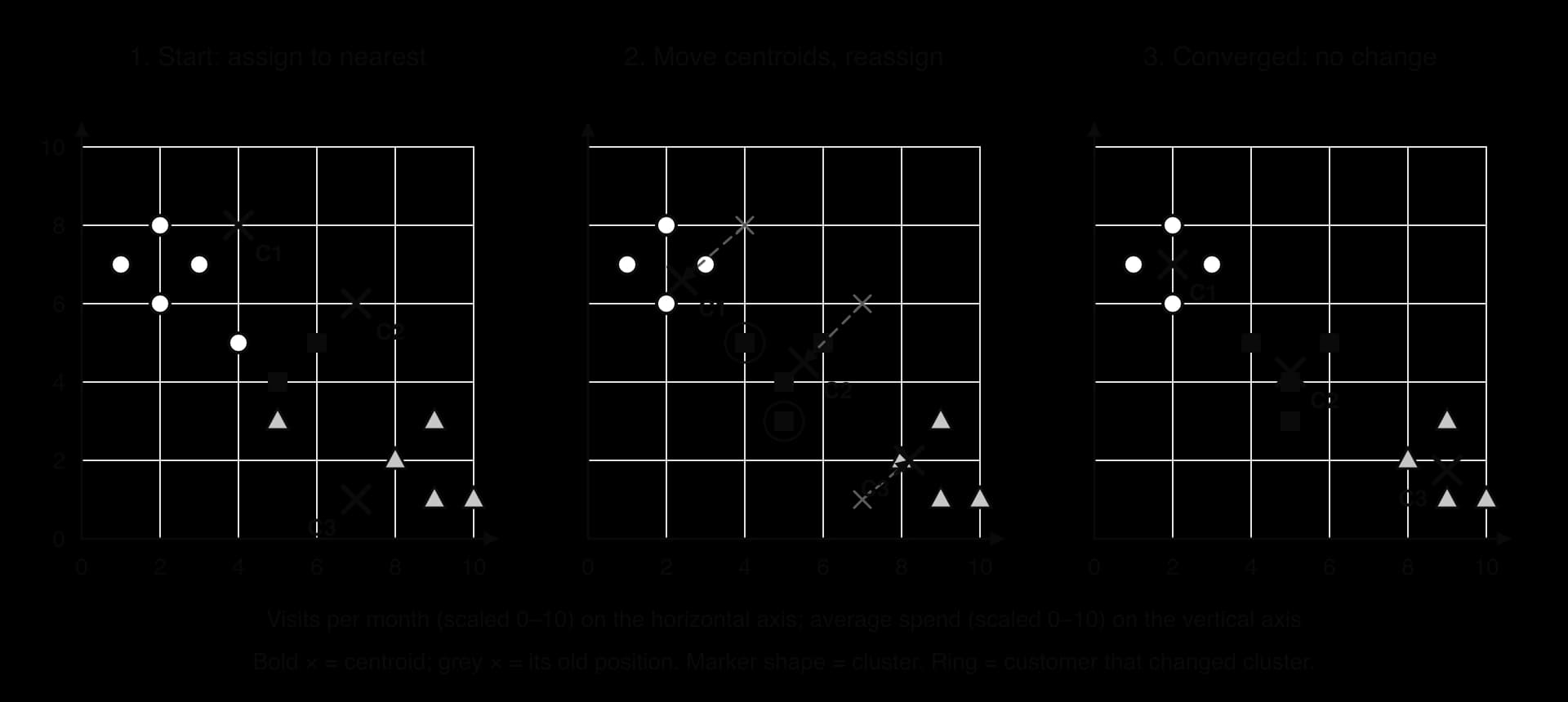
The final clusters can then be interpreted: C1 (few visits, high spend) might be labelled "occasional big spenders", C3 (many visits, low spend) "frequent small baskets" and C2 the customers in between. The shop might send the first group offers on premium products and the second a loyalty reward for visits. These labels are a human interpretation, since k-means only reports which customers are close together.

Choosing k: the elbow method

The number of clusters must be chosen before k-means runs. Too few merges groups that are really different; too many splits natural groups into fragments. One guide is the within-cluster sum of squares (WCSS): the total of the squared distances from each point to its centroid. WCSS always falls as $k$ rises (with $k$ equal to the number of points it reaches 0), so the lowest WCSS is not the goal. The elbow method plots WCSS against $k$ and looks for the point where adding another cluster stops giving a large improvement.

Source: computed for the twelve hypothetical customers, taking the best of every possible set of data points as starting centroids for each k.

The elbow is not always sharp, so domain knowledge also guides the choice: a marketing team that can only run three campaigns may want $k = 3$ whatever the plot shows.

Strengths and limitations of k-means

k-means is simple, fast (each iteration takes time proportional to the number of points × $k$) and works on large data sets. Its weaknesses follow from how it works:

• Sensitive to the starting centroids. Starting the twelve customers from centroids at (1, 7), (2, 6) and (5, 4) converges to a different, worse grouping, with a WCSS of 44.1 instead of 13.5. Practical systems run k-means several times from different starts and keep the best result.

• k must be chosen in advance, by the elbow method or domain knowledge.

• Sensitive to scale and outliers. Distances are dominated by features with large ranges, so features must be scaled (subtopic A4.2), and a single outlier can drag a centroid away from its group.

• Assumes compact, roughly round clusters of similar size. Long, curved or nested clusters are split wrongly; other algorithms, such as hierarchical clustering or DBSCAN, handle such shapes better.

Association rules

Some of the most useful patterns in large data sets are co-occurrences, things that tend to happen together. Market basket analysis looks for products bought together; police analysts look for offences that occur in the same areas; doctors look for symptoms that appear together. Association rule learning is the data mining technique that finds such patterns and measures how strong they are.

Antecedents, consequents and itemsets

In the rule {coffee} → {croissant}, the left-hand side is the antecedent (the "if" part) and the right-hand side is the consequent (the "then" part). Both are itemsets: sets of one or more items. A rule such as {coffee, croissant} → {juice} has a two-item antecedent.

The arrow has a direction. {coffee} → {croissant} and {croissant} → {coffee} are different rules, and they can have very different strengths.

An itemset is called frequent when it appears in at least a chosen minimum fraction of the records. Finding the frequent itemsets is the expensive part of association rule mining; turning them into rules is quick.

Support, confidence and lift

Three measures describe a rule $X \rightarrow Y$, where $N$ is the total number of records (transactions).

Support measures how common the pattern is: the fraction of all transactions that contain every item in both $X$ and $Y$. A rule with very low support may be a coincidence and is of little business value even if it is reliable.

Confidence measures how reliable the rule is: of the transactions that contain $X$, the fraction that also contain $Y$. It is an estimate of the probability of $Y$ given $X$.

Confidence alone can mislead. If almost every customer buys coffee, then {anything} → {coffee} has high confidence simply because coffee is popular. Lift corrects for this by comparing the confidence with how often $Y$ occurs anyway:

Worked transaction table

A hypothetical school café records ten transactions.

Counting each item gives its support: coffee 6/10 = 0.6, croissant 6/10 = 0.6, muffin 5/10 = 0.5, juice 4/10 = 0.4 and tea 3/10 = 0.3. The table of rules applies the three formulas.

Two features of the table hold in general. Support and lift are the same in both directions for a pair, but confidence is not: two-thirds of tea buyers buy a muffin, but only two-fifths of muffin buyers buy tea. A lift below 1, as for croissants and muffins, shows that customers tend to choose one or the other, which is useful in its own right because the two may be substitutes.

Mining rules efficiently: the Apriori algorithm

A shop with 1,000 products has nearly 500,000 possible pairs and over 166 million possible triples, so counting every itemset in millions of transactions is impractical. The Apriori algorithm, published by Rakesh Agrawal and Ramakrishnan Srikant in 1994, avoids most of this work by using the fact that every subset of a frequent itemset must also be frequent. Any itemset that contains an infrequent item (or infrequent pair) therefore cannot be frequent, so it never needs to be counted.

The Apriori process:

1. Set a minimum support and a minimum confidence.

2. Count single items; keep those with at least the minimum support.

3. Build candidate pairs only from frequent single items; count them and keep the frequent pairs.

4. Build candidate triples only from frequent pairs, and so on, until no new frequent itemsets appear.

5. From each frequent itemset, form rules and keep those whose confidence meets the minimum.

With a minimum support of 0.3, every other pair in the café data has support 0.2 or less, and every triple contains at least one of those infrequent pairs, so Apriori stops without counting any triple. The two rules from the frequent pair, {coffee} → {croissant} and {croissant} → {coffee}, both have confidence 0.83.

Interpreting rules: the crime analysis example

Association rules apply far beyond shopping. In crime analysis, each "transaction" might be a neighbourhood and month, and the "items" the types of incident recorded. A rule {vandalism} → {theft} with high confidence and a lift above 1 would mean that areas with vandalism are more likely than average to experience theft as well, and police could use it to plan patrols or prevention work where vandalism is rising.

The interpretation needs care. A rule shows co-occurrence, not cause: vandalism does not necessarily lead to theft, and both may stem from a third factor such as poor street lighting or an empty building. Recorded crime also reflects where police already patrol, so rules mined from it can direct more patrols to the same areas, find more crime there and reinforce the pattern, a feedback loop that raises questions of fairness covered in subtopic A4.4.

Reinforcement learning

In supervised learning every example comes with the right answer. Many decision problems have no such answers: nobody can label the "correct" move in every position of a board game, or the correct speed for a robot at every instant. Reinforcement learning tackles these problems by trial and error. An agent acts in an environment, receives a reward or penalty, and gradually learns which actions lead to the most reward over time.

The agent–environment loop

At each time step the agent observes the state of the environment, chooses an action, and the environment responds with a reward and a new state. The cycle then repeats, as the diagram of the reinforcement learning loop shows.

The state of a robot vacuum cleaner might be its position, the map of cleaned areas and its battery level; the state of a board game is the position of every piece. In each state the agent selects one of the moves open to it.

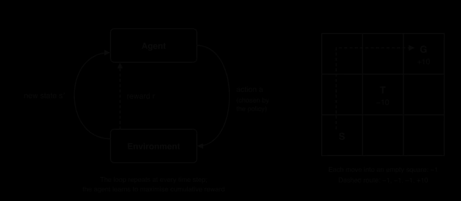
The agent's strategy, the rule that tells it which action to take in each state, is its policy. Learning in reinforcement learning means improving the policy. A policy can be a simple table (in state A take action 2) or, in large problems, a neural network that takes the state as input and outputs a score for each action.

Cumulative reward

The agent aims to maximise its cumulative reward over the whole task, even if that means accepting a smaller reward on the next step. Many good actions pay off only later: a chess player sacrifices a piece to win the game, and a robot takes a longer path to avoid a hazard. An agent that maximised only the next reward would miss these.

With a discount factor $\gamma$ (gamma), a reward received $t$ steps in the future is multiplied by $\gamma^t$:

A discount factor near 1 makes the agent far-sighted; near 0 it cares mostly about immediate reward. Discounting also favours reaching a goal quickly, because the same final reward is worth less when it arrives later.

Exploration and exploitation

An agent that has found one action with a good reward has a choice at every step. It can exploit what it knows and take the best action found so far, or explore by trying an action whose value is still uncertain, which may turn out to be better (or worse).

Too much exploitation leaves the agent stuck with the first reasonable strategy it finds, never discovering a better one. Too much exploration wastes time on actions already known to be poor. A delivery robot that always takes the first route it found may never discover a quicker one; a robot that tries a random route every day never benefits from what it has learned.

The simplest way to balance the two is the epsilon-greedy strategy. With a small probability $\varepsilon$ (for example 0.1) the agent picks an action at random; otherwise it picks the action with the highest estimated value. Often $\varepsilon$ starts large, when the agent knows little, and is reduced as learning goes on.

Under ε-greedy the best-known action is chosen more often than $1 - \varepsilon$ of the time, because a random choice can also land on it. A hypothetical news app choosing between three headline styles with $\varepsilon = 0.1$ shows its current best style with probability $0.9 + 0.1 \times \tfrac{1}{3} = 0.93$

How the agent learns, and where it is used

As it acts, the agent keeps estimates of how much cumulative reward each action leads to from each state, and updates them after every reward: actions followed by high rewards become more likely, those followed by penalties less likely. A standard algorithm of this kind is Q-learning, which stores an estimated value for every state–action pair; when there are too many states for a table, a neural network estimates the values instead (deep reinforcement learning).

The same loop describes robots learning to walk or navigate, game-playing programs, traffic-light controllers rewarded for short queues, and recommendation systems rewarded for clicks. The best-known example is AlphaGo, developed by DeepMind, which beat the professional Go player Lee Sedol by four games to one in Seoul in March 2016. AlphaGo's neural networks first learned to imitate moves from a database of about 30 million moves from human expert games, then improved by playing large numbers of games against copies of itself, using reinforcement learning with the win or loss at the end of each game as the reward.

Source: "AlphaGo versus Lee Sedol" and "AlphaGo", Wikipedia, accessed 2026.

Genetic algorithms

Some problems call for a search for the best design or plan among an astronomically large number of possibilities. A genetic algorithm borrows the idea of evolution by natural selection to search such spaces: it keeps a population of candidate solutions, lets the better ones "breed", adds small random changes, and repeats over many generations. Strictly it is an optimisation and search method rather than learning from labelled data, but it is grouped with machine learning because performance improves automatically from feedback.

Optimisation problems and the travelling salesperson

An optimisation problem asks for the best solution among many possible ones, judged by a measurable goal: the shortest route, the cheapest timetable that breaks no rules, the lightest bridge that carries a given load.

The classic example is the travelling salesperson problem (TSP): given a list of cities and the distance between each pair, find the shortest route that visits every city exactly once and returns to the start. It models delivery rounds, circuit-board drilling and school-bus routes.

The difficulty is the number of routes. With $n$ cities, fixing the start city and counting each route and its reverse once gives

For 5 cities that is 12 routes; for 10 cities, 181,440; for 20 cities, about $6.1 \times 10^{16}$. Checking every route (brute force) is possible for small $n$ but impractical for a delivery company with 50 stops. A genetic algorithm does not guarantee the best route, but it usually finds a very good one in a reasonable time.

The parts of a genetic algorithm

Each candidate solution is encoded as a chromosome. For the TSP, a natural chromosome is the order in which the cities are visited, such as ADCBE. The set of chromosomes held at one time is the population.

A population typically holds 50 to several hundred chromosomes, generated at random at the start so that they cover many parts of the search space.

A fitness function scores how good each chromosome is. For the TSP, a shorter route is better, so a common choice is fitness = 1 ÷ route length (or a constant divided by the length). The fitness function is the only place where the problem's goal enters the algorithm, so designing it well is most of the work.

Selection chooses which chromosomes become parents, favouring fitter ones while still giving weaker ones some chance, which keeps the population varied. In roulette-wheel selection each chromosome's chance of being picked is its fitness divided by the total fitness of the population. In tournament selection a few chromosomes are picked at random and the fittest of them becomes a parent.

Crossover combines two parents into a child that inherits parts of each, in the hope of joining good features of both. Simply cutting two routes and joining the pieces would repeat some cities and drop others, so routes use an order-preserving crossover: a slice of parent 1 is copied into the child in the same positions, and the gaps are filled with the remaining cities in the order they appear in parent 2.

Mutation makes a small random change to a child, such as swapping two cities. It keeps the population diverse and lets the search reach routes that crossover alone could never produce. The mutation rate is kept low (often around 1% per gene), because heavy mutation turns the search into a random one.

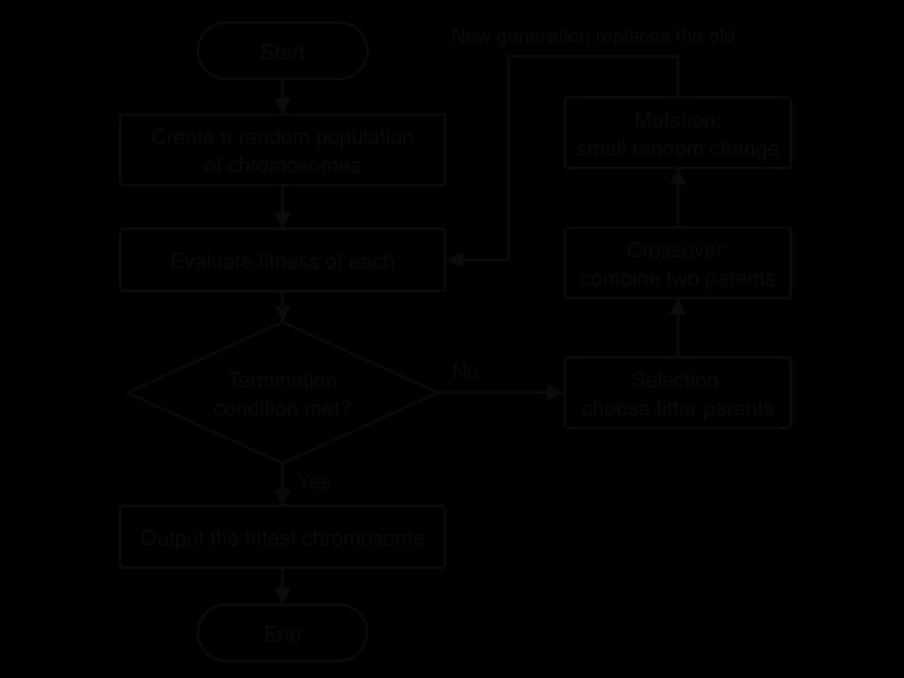
The new chromosomes form the next generation, which is evaluated with the fitness function in turn. The cycle stops when a termination condition is met.

Common termination conditions are a fixed number of generations, a time limit, a good-enough solution (a route under a target length), or no improvement in the best fitness for a set number of generations.

The flowchart of the genetic algorithm cycle puts the steps together.

A worked route-planning example

A hypothetical courier must visit five depots, A to E, starting and ending at A. The distance table gives the road distance in km between each pair.

A starting population of four random routes is scored by measuring each route, including the return to A. The fitness is 100 ÷ route length, so shorter routes score higher.

Order crossover of ACBDE (parent 1) with ABDCE (parent 2), keeping parent 1's last two cities D and E in place, fills the first three positions with A, B and C in the order they appear in parent 2. The child ABCDE measures 4 + 5 + 4 + 6 + 3 = 22 km, shorter than either parent and in fact the shortest of all 12 possible routes. A swap mutation of its third and fourth cities gives ABDCE (29 km), which is worse; most random changes to a good solution are harmful, and selection discards them in the next generation.

Applications and limitations

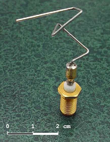
Genetic algorithms suit problems where a solution can be encoded and scored but the search space is too large to explore exhaustively and has no simple structure to use: vehicle routing, school timetabling, factory scheduling, choosing hyperparameters for other ML models, and engineering design. A well-known design example is the antenna of NASA's Space Technology 5 mission. Its shape was found by an evolutionary algorithm, which generated antenna shapes, scored them against the mission's requirements and bred the best; the resulting antenna flew after the mission's launch on 22 March 2006, the first artificially evolved object to fly in space.

The limitations of genetic algorithms follow from the method. A genetic algorithm gives no guarantee of finding the optimal solution, and it may converge prematurely on a good but not best one when the population loses diversity. It has many hyperparameters (population size, mutation rate, selection method) that affect results, it is random, so two runs can give different answers, and evaluating the fitness of thousands of candidates can be slow if each evaluation is a costly simulation.

Artificial neural networks

An artificial neural network (ANN) is a model built from many simple, connected processing units, loosely inspired by the neurons of the brain. Each unit does very little: it multiplies its inputs by weights, adds them up and passes the result through a simple function. Connected in layers and trained on large amounts of data, these units can model patterns far too complex to write down as rules, so neural networks are used for classification (spam or not spam), regression (tomorrow's demand) and pattern recognition in images, sound and text.

The perceptron: a single artificial neuron

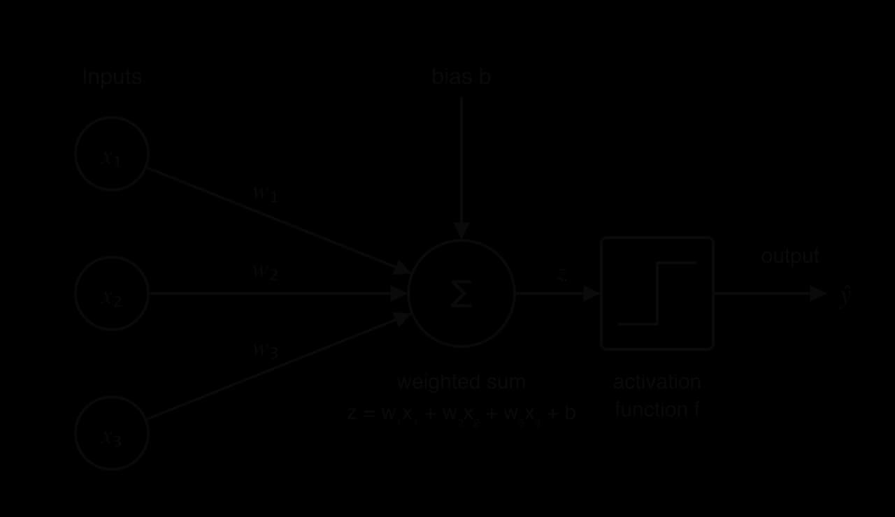
The building block of every neural network is the artificial neuron. The earliest and simplest form, the perceptron, takes several numerical inputs and produces one output.

Each input $x_i$ is multiplied by a weight $w_i$, which sets how strongly, and in which direction, the input affects the output: a large positive weight raises the output, a negative weight lowers it, and a weight near zero makes the input almost irrelevant. The weights are the model parameters that training adjusts.

The neuron then adds up the weighted inputs and one extra number, the bias, which shifts the point at which the neuron "fires": the neuron can produce a positive output even when all inputs are zero, or stay off unless the inputs are large. The bias plays the role of the intercept in the equation of a straight line.

The result is the weighted sum, often written $z$:

Finally the weighted sum goes through an activation function $f$, which gives the neuron's output $\hat{y} = f(z)$. Rosenblatt's perceptron used a step function: the output is 1 if $z > 0$ and 0 otherwise. (Some books use $z \ge 0$

The sketch of a perceptron shows every part that must be labelled: inputs, weights, bias, summation, activation function and output.

What a single perceptron can and cannot learn

With two inputs, a perceptron's decision boundary is the line $w_1 x_1 + w_2 x_2 + b = 0$

The logic gates of subtopic A1.2 (Data representation and computer logic) show the limit. AND is linearly separable: with $w_1 = w_2 = 1$ and $b = -1.5$, only the input (1, 1) gives a positive weighted sum (0.5). OR is too: with

Multi-layer perceptrons

A multi-layer perceptron (MLP) arranges neurons in layers. The input layer receives the features, one neuron per feature, and passes them on without calculation. One or more hidden layers transform them. The output layer produces the prediction.

The input layer's size is fixed by the data: a model that reads 28 × 28 pixel greyscale images has 784 input neurons, one per pixel.

Hidden layers are called hidden because their values are never seen in the training data: only inputs and outputs are. Each hidden neuron combines the outputs of the previous layer into a new feature, and with several hidden layers the network can build features of features.

The output layer has one neuron per value to predict: one for a regression output or a yes/no probability, or one per class in a multi-class problem.

In an MLP every neuron in one layer is connected to every neuron in the next, with a separate weight on each connection; there are no connections between neurons in the same layer, and no connections that skip backwards. Such a layer is fully connected.

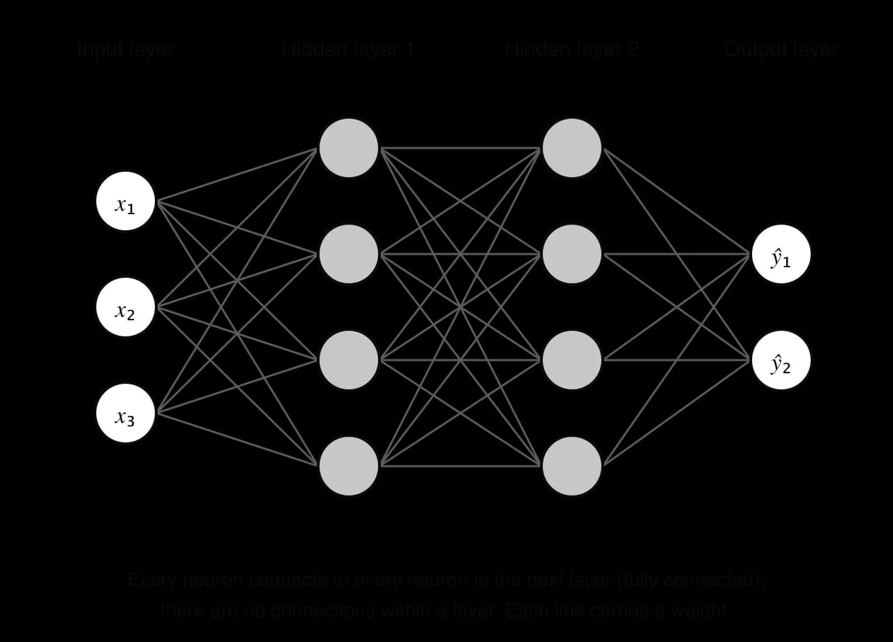
Between two fully connected layers there is one weight per pair of neurons, plus one bias per neuron in the receiving layer. The network in the diagram therefore has $(3 \times 4 + 4) + (4 \times 4 + 4) + (4 \times 2 + 2) = 46$

Activation functions in multi-layer networks

The step function is unsuitable inside an MLP for two reasons. Its output jumps from 0 to 1, so a small change to a weight usually changes nothing and then suddenly changes everything, which gives the training algorithm no information about which direction improves the network. And if every neuron were linear (no activation function, or $f(z) = z$), a stack of layers would collapse into one linear function, no more capable than a single layer. Hidden layers therefore use smooth, non-linear activation functions, compared in the graph of activation functions.

ReLU (rectified linear unit) is now the default for hidden layers because it is very cheap to compute and, for positive inputs, its slope never shrinks; sigmoid and tanh flatten out for large inputs, which slows learning in deep networks (the vanishing gradient problem). Softmax turns the output layer's raw scores into probabilities: scores of 2.0, 1.0 and 0.1 for "cat", "dog" and "car" become 0.66, 0.24 and 0.10.

How a neural network learns

Training adjusts the weights and biases so that the network's outputs match the labels in the training data. In outline, it runs as follows:

1. Forward pass: an example's features go through the network, layer by layer, to produce a prediction.

2. Loss: a loss function measures how wrong the prediction is.

3. Backward pass: backpropagation works out how much each weight contributed to the error.

4. Update: gradient descent changes each weight slightly in the direction that reduces the loss.

5. Repeat for every example, many times over the training data.

The loss function defines what "wrong" means. For regression the usual choice is mean squared error (MSE), the mean of the squared residuals (for the bakery line, $48 \div 6 = 8$). For classification it is cross-entropy, $-\ln(p)$, where $p$ is the probability the network gave to the correct class: a confident correct answer ($p = 0.85$

Backpropagation calculates, for every weight at once, whether a slightly larger value of that weight would raise or lower the loss, and by how much. Gradient descent then uses these results.

The size of each step is set by the learning rate, a hyperparameter. Gradient descent is often pictured as walking downhill in fog: the walker cannot see the valley floor, but can feel which way the ground slopes and take a step that way. Too large a learning rate overshoots the valley and the loss jumps about; too small a rate makes training extremely slow.

One complete pass through all the training data is an epoch; training usually lasts many epochs. The data is normally processed in small batches (for example 32 examples), with one weight update per batch; the batch size is another hyperparameter.

The perceptron's own learning rule shows the same loop in its simplest form. For each training example it computes the output, finds the error (target − output), and changes each weight by learning rate × error × input and the bias by learning rate × error. Trained on the AND function from zero weights with a learning rate of 0.1, it reaches weights 0.2 and 0.1 and a bias of −0.2 after five epochs, and the sixth epoch produces no errors. These values differ from the hand-chosen 1, 1 and −1.5 but separate the classes just as well: only the input (1, 1) gives a positive weighted sum (0.1). Trained on XOR instead, the rule never completes an epoch without errors, because no straight line separates the XOR classes.

YouTube

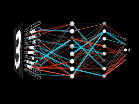
The 3Blue1Brown video uses a 784-input network for handwritten digits, the same input size as the 101,770-parameter network, and suggests why hidden layers might learn edges, then loops and lines, then whole digits. That idea of layers building more abstract features is designed directly into convolutional neural networks.

Convolutional neural networks

An MLP can classify images, but poorly and expensively. It treats each pixel as an unrelated input, so its structure ignores the fact that neighbouring pixels belong together, and a cat in the top-left corner and the same cat in the bottom-right are completely different inputs. It also needs a huge number of weights: a 224 × 224 colour image has $224 \times 224 \times 3 = 150\,528$ input values, so a first hidden layer of 1,000 neurons alone would need over 150 million weights. A convolutional neural network (CNN) is designed for grid-shaped data such as images and avoids both problems.

The input: an image as numbers

To a CNN, an image is a grid of numbers. A greyscale image has one value per pixel (for example 0 for black to 255 for white); a colour image has three channels (red, green and blue), so it is a block of height × width × 3 numbers. The number of possible values per pixel depends on the colour depth. Before training, pixel values are usually scaled to the range 0 to 1.

Convolutional layers and kernels

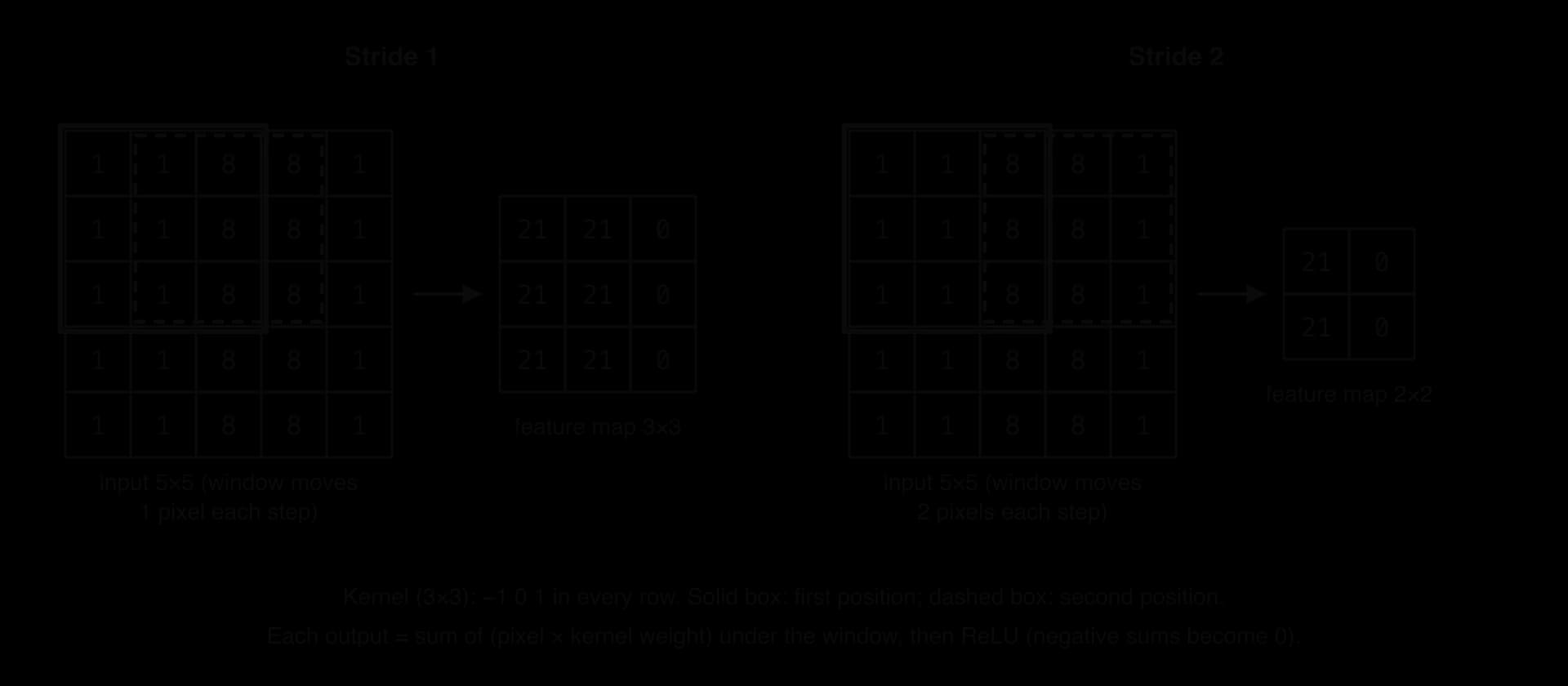
A convolutional layer slides small grids of weights, called kernels or filters, across the image. At each position the kernel's weights are multiplied by the pixel values under it and the products added up (plus a bias) to give one number. The grid of numbers produced as the kernel moves over the whole image is a feature map: it shows where in the image the kernel's pattern appears.

A kernel is typically 3 × 3 or 5 × 5 (with the same depth as its input). Its weights are not designed by hand: they start random and are learned by backpropagation, so training determines which patterns each kernel detects.

Because the same kernel is used at every position, a pattern is detected wherever it appears, and the layer needs only the kernel's few weights, not one weight per pixel. This weight sharing is the main reason CNNs need far fewer parameters than MLPs.

Two hyperparameters control how the kernel moves. The stride is the number of pixels the kernel moves at each step. A stride of 1 visits every position; a stride of 2 skips every other position, roughly halving the width and height of the feature map, which saves computation but loses detail.

A kernel cannot be centred on an edge pixel without hanging over the border, so each convolution shrinks the image and uses edge pixels less than central ones. Padding adds a border of extra pixels, usually zeros, around the input, so that the feature map can keep the input's width and height.

The diagram of a kernel at stride 1 and stride 2 shows a 3 × 3 vertical-edge kernel sliding over a 5 × 5 image with no padding.

Activation and pooling layers

After each convolution, an activation function, almost always ReLU, is applied to every value of the feature map. Without it, a stack of convolutional layers would again collapse into one linear operation and could not learn complex shapes.

A pooling layer then shrinks each feature map. It slides a small window (usually 2 × 2 with stride 2) over the map and keeps one value per window: the largest (max pooling) or the mean (average pooling). Max pooling a 4 × 4 map with rows 1 3 2 0 / 5 6 1 2 / 0 2 9 4 / 3 1 7 8 gives the 2 × 2 map 6 2 / 3 9; average pooling gives 3.75 1.25 / 1.5 7.

Pooling has no weights to learn; it is a fixed operation. It cuts the amount of data the next layers must process (a 2 × 2 pool keeps a quarter of the values), and it makes the network tolerant of small shifts: if an edge moves by one pixel, the maximum of its window is often unchanged.

Fully connected and output layers

After several rounds of convolution, activation and pooling, the final feature maps are flattened into one long list of numbers and passed to one or more fully connected layers, exactly as in an MLP. These layers combine the detected features ("whiskers here, pointed ears there") into a decision. The output layer has one neuron per class and uses softmax to turn its scores into probabilities, and the class with the highest probability is the prediction.

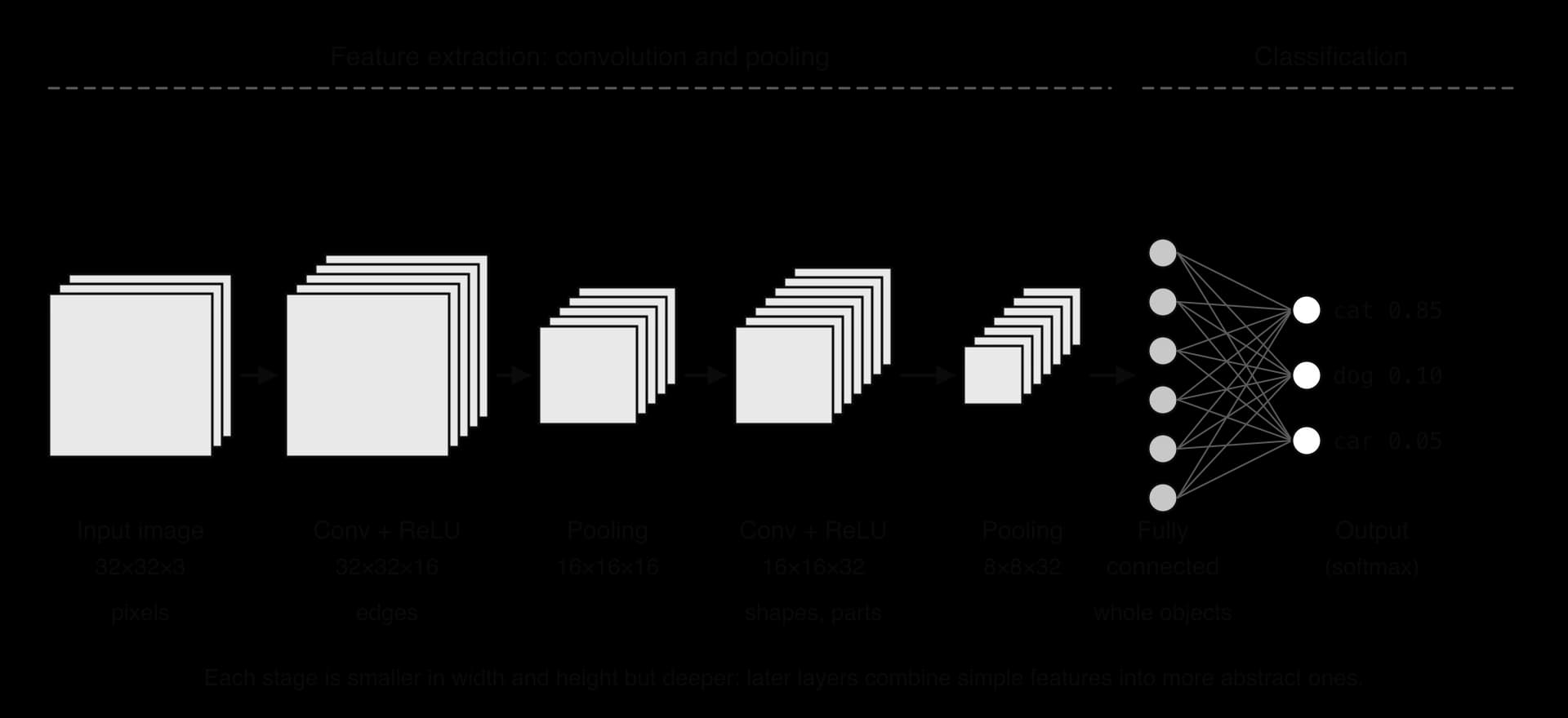
The example pipeline uses padding in its convolutional layers, so convolution keeps the width and height (32 × 32) while the 16 kernels give 16 feature maps; each pooling layer halves the width and height. The final 8 × 8 × 32 = 2,048 values are flattened for the fully connected layer.

Spatial hierarchies and receptive fields

The layers of a CNN learn a spatial hierarchy of features. Kernels in the first layer, which see only tiny patches of pixels, learn simple features such as edges and colour changes. The second layer's kernels look at the first layer's feature maps, so they respond to combinations of edges: corners, curves, textures. Deeper layers combine those into parts (an eye, a wheel) and then whole objects. Nobody programs this hierarchy; it emerges from training because it is the most useful way to reduce the loss.

The hierarchy works because each layer's receptive field grows. A neuron in the first 3 × 3 convolutional layer sees a 3 × 3 patch of the image; a neuron in a second 3 × 3 layer sees a 3 × 3 patch of the first layer's map, which covers 5 × 5 pixels of the original image; pooling and larger strides make the field grow faster still. By the deepest layers a single neuron is influenced by most of the image.

How design choices affect a CNN

Weight sharing makes a large difference to the number of parameters. A first convolutional layer with 16 kernels of size 3 × 3 on a colour image has $16 \times (3 \times 3 \times 3 + 1) = 448$ parameters (27 weights and one bias per kernel), whatever the size of the image. A fully connected layer of 1,000 neurons on the same 32 × 32 × 3 image needs $3\,072 \times 1\,000 + 1\,000 = 3\,073\,000$

AlexNet

The CNN that made the approach famous was AlexNet, built by Alex Krizhevsky, Ilya Sutskever and Geoffrey Hinton at the University of Toronto. It won the 2012 ImageNet Large Scale Visual Recognition Challenge, which asks for 1,000 categories of object to be recognised, with a top-5 error rate of 15.3% (the correct class was missing from its five best guesses for 15.3% of test images), more than 10.8 percentage points better than the runner-up. Its design is the standard pipeline: five convolutional layers, some followed by max-pooling layers, then three fully connected layers, with ReLU activations, in total about 60 million parameters.

Source: "AlexNet", Wikipedia, accessed 2026; Krizhevsky, Sutskever and Hinton, 2012.

AlexNet's design shows these trade-offs in practice. ReLU rather than tanh or sigmoid let a network of this depth train in a practical time, max pooling reduced the size of the feature maps between layers, and the large number of parameters needed the 1.2 million labelled training images of ImageNet to avoid severe overfitting.

YouTube

The Computerphile video follows the same steps as the vertical-edge example: a kernel produces a feature map, ReLU removes negative values, and pooling shrinks the map before the next layer.

Model selection and comparison

No single algorithm is best for every problem. Each approach makes assumptions about the data: linear regression assumes a straight-line relationship, k-NN assumes that nearby points share a class, k-means assumes round clusters, a CNN assumes that local patterns in a grid matter. When the assumptions fit the data, the model does well; when they do not, it does badly, however carefully it is tuned. Model selection is the process of choosing the approach, and then the specific model, that best suits the problem.

The formal version of the first sentence is the no free lunch theorem, proved by David Wolpert and William Macready in the 1990s. Averaged over every possible problem, all learning and search algorithms perform equally well; an algorithm that does better on some kinds of problem must do worse on others. In practice this means that model choice has to be justified by the particular problem and data, and checked by experiment.

Factors that guide the choice

The nature of the problem rules most approaches in or out at once. A continuous output needs regression, a category needs classification, unknown groups need clustering, co-occurrences need association rules, a sequence of decisions with delayed reward needs reinforcement learning, and a search through a huge space of designs or plans suits a genetic algorithm. Supervised methods also need labelled data, which can be expensive to obtain. The characteristics of the data and the desired outcomes then narrow the choice:

• Size of the data set. Deep networks need large amounts of data; with a few hundred examples, a decision tree or linear regression usually generalises better.

• Dimensionality and type. Images and sound suit CNNs; tables of a few meaningful features suit trees, regression or k-NN, which degrades with many features.

• Shape of the relationship. A linear model cannot capture a curved relationship; an MLP or a tree can.

• Noise and imbalance. k-NN with small $k$ and deep trees are sensitive to noise; class imbalance calls for precision, recall and F1 rather than accuracy when comparing models.

• Interpretability. In medicine, lending and law, people affected by a decision may need to know why it was made. Decision trees and linear regression can be explained; a deep network is close to a black box.

• Cost and speed. Training a deep network may need GPUs for days, k-NN predicts slowly on large data, and a model running on a phone must be small and fast.

Comparing models fairly

Once there are candidates, they must be compared on equal terms: the same training data, the same validation data (or the same cross-validation folds), and the same metric, chosen to match the costs of the problem. A model that looks better on one random split may simply have been lucky, so cross-validation, which averages over several splits, gives a fairer comparison. The final, chosen model is evaluated once on the untouched test set.

A practical strategy is to start with a simple baseline (always predicting the most common class, or a linear model) and to accept a more complex model only if it beats the baseline by enough to justify its extra cost and loss of interpretability.

Case study: The Netflix Prize

Between 2006 and 2009 the film-rental and streaming company Netflix ran an open competition, the Netflix Prize, offering US$1,000,000 to the first team that could predict how users would rate films 10% more accurately than its own recommendation system, Cinematch. The competition shows collaborative filtering, held-out test data and model comparison at a large scale. (The size and sparsity of its data set are discussed in subtopic A4.2, Data preprocessing.)

The data and the task

Teams received over 100 million past ratings (1 to 5 stars) and had to predict the hidden ratings in a qualifying set of about 2.8 million user–film pairs. Accuracy was measured by root mean squared error (RMSE), the square root of the mean squared difference between predicted and actual ratings. Cinematch scored 0.9525 on the test data, so the target was about 0.857.

Source: "Netflix Prize", Wikipedia, accessed 2026, from Bennett and Lanning, "The Netflix Prize", 2007.

The split was designed against overfitting. Teams could submit many times and see their quiz-set score, so a team could, in principle, tune its models to the quiz set. The prize was decided on the hidden test set, whose scores no team ever saw, in the same way that a final test set is kept untouched during hyperparameter tuning.

How the winning approach worked

The leading teams combined many different models: neighbourhood methods of the k-NN kind (users or films with similar rating patterns), matrix factorisation methods that describe each user and film by a small number of learned features, and neural networks. Each model captured something the others missed, and blending their predictions reduced the error further than any single model could. On 21 September 2009 the grand prize went to BellKor's Pragmatic Chaos, a team formed by merging earlier competitors, whose predictions were 10.06% more accurate than Cinematch's (a test RMSE of 0.8567). A rival merged team, The Ensemble, matched that test score but had submitted 20 minutes later.

Evaluation

The competition showed the value of comparing models openly on the same data and the same metric: thousands of teams could be ranked fairly because everyone was scored on one hidden test set by one formula. The winning blend also reflects the no free lunch theorem, since different algorithms were good at different parts of the problem.

The prize also showed the limits of accuracy as the only goal. Netflix reported in 2012 that the extra accuracy of the final prize-winning blend did not seem to justify the engineering effort of putting it into its production system, and that its business had meanwhile moved towards streaming, where what people choose to watch matters more than the stars they award. Cost, speed, maintainability and changing requirements are part of model selection alongside accuracy.

Source: Netflix Technology Blog, "Netflix Recommendations: Beyond the 5 stars", April 2012.

Exam focus

Machine learning approaches are HL only. They are examined in Paper 1 Section A as extra question parts on HL papers, often attached to a scenario that the SL parts have already introduced, and they can support Section B answers when the case study involves machine learning. No code is needed: questions ask you to calculate, trace and interpret, and to explain and justify choices in context.

The statements use Explain (linear regression, classification, hyperparameter tuning, model selection), Describe (clustering, association rules, reinforcement learning, genetic algorithms, CNNs) and Outline (ANNs, including sketches). Recurring question shapes:

• Calculate precision, recall, F1 or accuracy from a confusion matrix, or support, confidence and lift from a transaction table (2–4 marks).

• Determine a k-NN classification from a small table of points (3–4 marks), or trace k-means iterations or a case through a decision tree.

• Explain the meaning of a slope, intercept or r² in context (2 marks each).

• Sketch a perceptron or an MLP with the required labels (3–4 marks).

• Describe pooling, the exploration–exploitation trade-off, or how a genetic algorithm could plan routes (3–6 marks).

• Explain why one model would be chosen over another for a scenario (4–6 marks), often a decision tree against a neural network.

"Describe" and "explain" demand different answers. To describe k-means, give the steps in order (choose k, place centroids, assign, update, repeat until convergence). To explain why a high $k$ in k-NN causes underfitting, give the mechanism: many distant points vote, so local patterns are outvoted by the overall majority class.

Sketches are marked on their labelled parts. A perceptron needs inputs, weights, a bias, the weighted sum, the activation function and the output; an MLP needs an input layer, at least one hidden layer and an output layer, with every neuron joined to every neuron in the next layer and none within a layer.

Practice questions

1. State the difference between a model parameter and a hyperparameter, giving one example of each. [2]

2. A regression model predicts the price of a used car (in thousands of dollars) from its age in years: $\hat{y} = 24 - 1.8x$, $r^2 = 0.72$

Summary

• Linear regression fits $\hat{y} = b_0 + b_1x$ by least squares; the slope is the change in $y$

Self-check

• To do:

  I can interpret the slope, intercept and r² of a regression equation in context, and make a prediction.

• To do:

  I can explain why extrapolation is unreliable and why correlation does not prove causation.

• To do:

  I can classify a new point with k-NN from a table of data, showing a distance table and the vote.

• To do:

  I can explain the effect of a small and a large k, and why features must be scaled.

• To do:

  I can trace a new case through a decision tree and calculate the Gini impurity of a split.

• To do:

  I can construct a confusion matrix and calculate accuracy, precision, recall and F1 score.

• To do:

  I can choose the right metric for a scenario and explain why accuracy misleads with imbalanced classes.

• To do:

  I can distinguish hyperparameters from model parameters and describe how tuning uses validation data and cross-validation.

• To do:

  I can recognise overfitting and underfitting from training and validation results or a learning curve.

• To do:

  I can trace k-means iterations by hand and use an elbow plot to choose k.

• To do:

  I can calculate support, confidence and lift and interpret an association rule in context.

• To do:

  I can describe the agent–environment loop, calculate a discounted cumulative reward and explain ε-greedy.