A4.2 Data preprocessing

Learning objectives

• Describe how the quality of data affects the performance of a machine learning model, and the significance of data cleaning. (HL only)

• Describe how outliers are detected with box plots, the interquartile range rule and z-scores, and how they are handled. (HL only)

• Describe how duplicate, incorrect, irrelevant and improperly formatted data are found and corrected. (HL only)

• Describe deletion, imputation and predictive modelling as ways of handling missing data. (HL only)

• Describe normalisation and standardisation, calculate scaled values, and explain why distance-based and gradient-based algorithms need them. (HL only)

• Describe the role of feature selection and distinguish filter, wrapper and embedded methods. (HL only)

• Describe the curse of dimensionality: overfitting, computational cost, sparsity, distance metrics, visualisation, sample size and memory. (HL only)

• Describe the importance of dimensionality reduction and ways of reducing the number of features while keeping the relevant information. (HL only)

Introduction

A machine learning (ML) model learns only from the examples it is given. Real data is collected by people, sensors and forms, so it arrives with typing errors, gaps, repeated rows, mixed units and columns that have nothing to do with the task. Data preprocessing turns this raw material into a clean, consistent table of numbers that a learning algorithm can use, and includes choosing which features (columns) are worth keeping at all. In most ML projects it takes more time than training the model.

The decisions made during preprocessing change the results. Deleting every unusual value can remove the very cases a fraud detector is meant to find; filling gaps with an average can make a group of patients look healthier than they are; leaving a column measured in thousands next to one measured in single digits can make a distance-based model ignore the smaller one completely.

YouTube

Data quality and why cleaning matters

A model is a summary of the patterns in its training data. If the data contains errors, the model learns the errors as if they were patterns. A blood-pressure reading typed as 1350 instead of 135 pulls an average upwards; a patient recorded twice counts double; a label entered wrongly trains the model on the wrong answer for that example. No choice of algorithm can recover information that was never in the data or correct a bias that the data does not reveal.

Data quality describes how fit a dataset is for its purpose. It has several dimensions, and a dataset can be strong in one and weak in another: every value can be correct (accurate) while a third of the rows are missing (incomplete).

Dimensions of data quality, each linked to the cleaning problem that it causes. The hospital examples are hypothetical.

How poor data harms a model

Poor data harms a model in three distinct ways. First, noise: random errors hide the real pattern, so the model needs more data to find it and fits less well. Second, bias: systematic errors push the model in one direction, such as a scale that always reads 2 kg heavy or a survey answered mostly by one age group, and more data does not fix this because every new row carries the same error. Third, false confidence: duplicates and leaked information make the model look more accurate in testing than it is in use, so a poor model is deployed.

Even well-known benchmark datasets contain errors. MNIST, a set of handwritten-digit images used to test image classifiers since the 1990s, has at least four wrongly labelled images in its original release. With 70,000 images, four wrong labels hardly change a model, but the same error rate in a small medical dataset of 200 patients would matter far more.

Source: "MNIST database", Wikipedia, accessed 2026.

The preprocessing pipeline

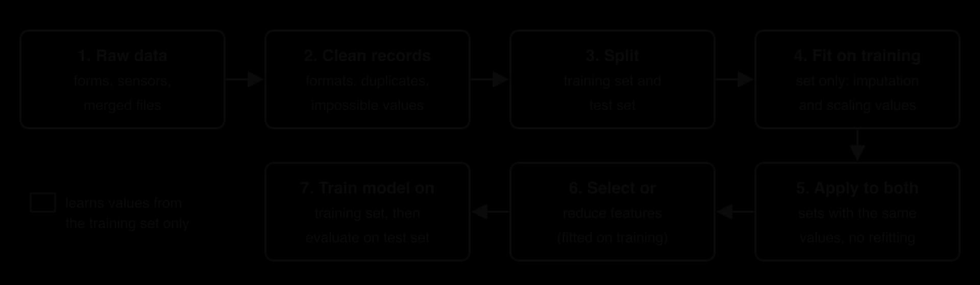
Preprocessing is a sequence of stages, and their order matters. Cleaning steps that fix individual records (correcting formats, removing duplicates, deleting impossible values) come first. The data is then split into a training set and a test set. Any step that learns a number from the data, such as the mean used for imputation or the minimum and maximum used for scaling, is calculated from the training set only and then applied unchanged to the test set. Feature selection and dimensionality reduction follow, and only then is the model trained.

Outliers

An outlier is a value far from the rest of the data. Some outliers are errors (a heart rate of 720 typed for 72); others are genuine but rare events (a heart rate of 180 during a medical emergency, a transaction of €40,000 on a card that usually spends €40). The difficulty is that both kinds look the same in the data, so the process has two separate steps: detect the unusual values, then decide, case by case, what each one is.

Outliers matter because many calculations are sensitive to them. The mean of a feature moves towards an outlier, the standard deviation grows, min-max scaling uses the outlier as one end of the range, and a model that minimises squared errors, such as linear regression, tilts its line towards it. A single extreme value can therefore change the model for every other record. When the outlier is the thing to be found (a fraudulent transaction, a failing machine), outlier detection becomes a task in its own right, called anomaly detection.

Seeing outliers: the box plot

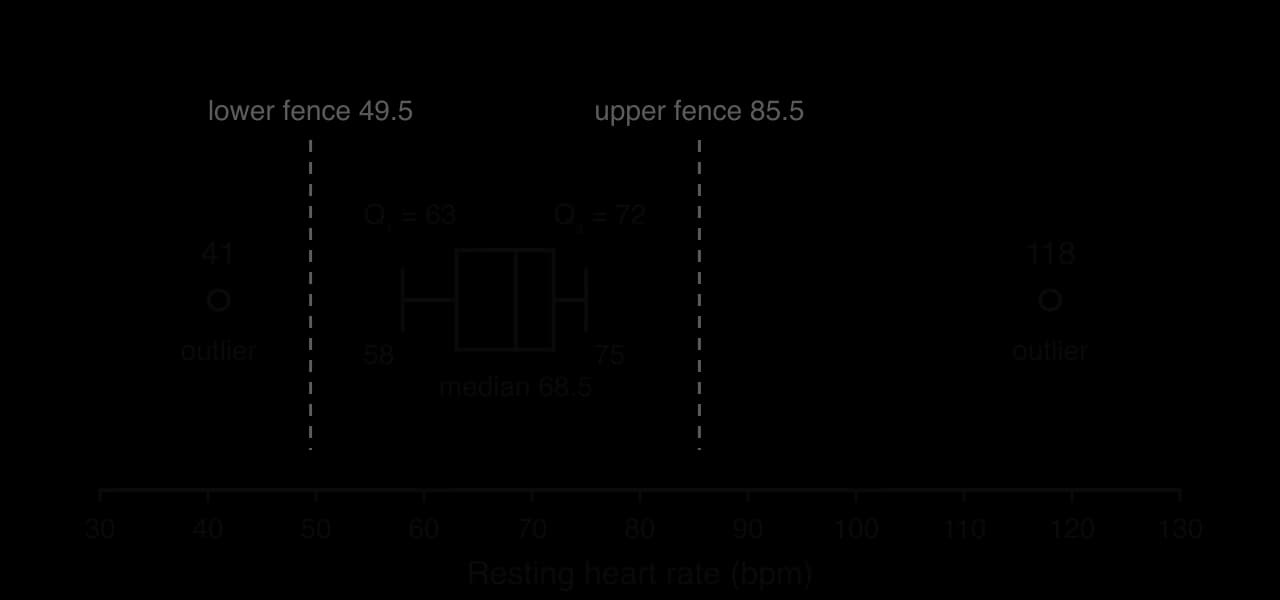
The quickest way to find outliers in one feature is to draw it. A box plot summarises a feature with five numbers: the lowest and highest values that are not outliers, the lower quartile, the median and the upper quartile. Values beyond the fences are drawn as separate points.

A hypothetical clinic records the resting heart rates of 12 patients, in beats per minute (bpm):

For two features at once, a scatter plot does the same job: a point far from the cloud of others is an outlier in the combination of features even when each value on its own looks ordinary. A height of 150 cm and a mass of 95 kg are each common, but together they are unusual and worth checking.

The interquartile range rule

The quartiles split the sorted data into four equal parts. A quarter of the values lie below the lower quartile $Q_1$, half below the median $Q_2$, and three-quarters below the upper quartile $Q_3$

The IQR rule draws two fences:

Any value outside the fences is flagged. The rule works well because the quartiles depend only on the middle of the data: an outlier, however extreme, cannot move $Q_1$ or $Q_3$ much, so it cannot hide itself by stretching the fences. The factor 1.5 is a convention; some analysts use 3 × IQR to flag only "far out" values.

Quartiles can be found in slightly different ways. The method used here sorts the data, splits it into a lower half and an upper half (leaving out the middle value when the count is odd) and takes the median of each half. Spreadsheets and programming libraries use other conventions, so their quartiles can differ slightly for small datasets. The fences change by only a little, and the same values are normally flagged whichever consistent method is used.

Z-scores

A second rule measures how many standard deviations a value lies from the mean. The standard deviation $\sigma$ is a measure of spread: roughly, the typical distance of a value from the mean $\mu$. It is the square root of the mean of the squared distances from the mean:

For data with a roughly bell-shaped (normal) distribution, about 99.7% of values have a z-score between −3 and 3, so a common rule flags any value with $|z| > 3$ as an outlier. Some analysts use a threshold of 2 or 2.5 when the dataset is small.

The z-score rule has a weakness the IQR rule does not. The mean and standard deviation are both calculated including the outliers, so an extreme value inflates $\sigma$ and drags $\mu$ towards itself, which shrinks its own z-score. This is called masking. In a small dataset the effect is severe: with $n$ values, no z-score can exceed $(n - 1) / \sqrt{n}$

The function iqr_fences sorts the data, finds the quartiles with a helper median and returns the two fences; z_scores calculates the mean and standard deviation with loops (the built-in sum and statistics functions are avoided so the method is visible) and returns every value's z-score.

import math


def median(values):
    # values must already be sorted
    n = len(values)
    middle = n // 2
    if n % 2 == 1:
        return values[middle]
    return (values[middle - 1] + values[middle]) / 2


def iqr_fences(data):
    values = sorted(data)
    n = len(values)
    lower_half = values[0:n // 2]
    upper_half = values[(n + 1) // 2:n]
    q1 = median(lower_half)
    q3 = median(upper_half)
    iqr = q3 - q1
    return q1 - 1.5 * iqr, q3 + 1.5 * iqr


def z_scores():
    total = 
     x  data:
        total = total + x
    mean = total / (data)
    squares = 
     x  data:
        squares = squares + (x - mean) ** 
    sd = math.sqrt(squares / (data))
    scores = []
     x  data:
        scores.append((x - mean) / sd)
     scores


heart_rates = [, , , , , , , , , , , ]
low, high = iqr_fences(heart_rates)
(, low, high)
 x  heart_rates:
     x < low  x > high:
        (, x)

scores = z_scores(heart_rates)
largest = 
 i  ((heart_rates)):
     (scores[i]) > :
        (, heart_rates[i])
     (scores[i]) > largest:
        largest = (scores[i])
(, (largest, ))

import java.util.Arrays;

public class Outliers {
    // values must already be sorted
    static double median(int[] values) {
        int n = values.length;
           n / ;
         (n %  == ) {
             values[middle];
        }
         (values[middle - ] + values[middle]) / ;
    }

     [] iqrFences([] data) {
        [] values = data.clone();
        Arrays.sort(values);
           values.length;
        [] lowerHalf = Arrays.copyOfRange(values, , n / );
        [] upperHalf = Arrays.copyOfRange(values, (n + ) / , n);
           median(lowerHalf);
           median(upperHalf);
           q3 - q1;
          [] {q1 -  * iqr, q3 +  * iqr};
    }

     [] zScores([] data) {
           ;
         ( x : data) {
            total = total + x;
        }
           total / data.length;
           ;
         ( x : data) {
            squares = squares + Math.pow(x - mean, );
        }
           Math.sqrt(squares / data.length);
        [] scores =  [data.length];
         (   ; i < data.length; i++) {
            scores[i] = (data[i] - mean) / sd;
        }
         scores;
    }

        {
        [] heartRates = {, , , , , , , , , , , };
        [] fences = iqrFences(heartRates);
        System.out.println( + fences[] +  + fences[]);
         ( x : heartRates) {
             (x < fences[] || x > fences[]) {
                System.out.println( + x);
            }
        }

        [] scores = zScores(heartRates);
           ;
         (   ; i < heartRates.length; i++) {
             (Math.abs(scores[i]) > ) {
                System.out.println( + heartRates[i]);
            }
             (Math.abs(scores[i]) > largest) {
                largest = Math.abs(scores[i]);
            }
        }
        System.out.println( + Math.round(largest * ) / );
    }
}

Both versions print the same result. The z-score loop prints nothing because no value passes the threshold, since masking hides both outliers from the z-score rule. The Java version copies the array with clone() before sorting so the caller's data keeps its original order; Python's sorted() returns a new list for the same reason. Python returns two values as a tuple, whereas Java returns an array of two double values.

Fences: 49.5 85.5
IQR outlier: 118
IQR outlier: 41
Largest |z|: 2.86

Deciding what to do with an outlier

Detection only produces a list of suspicious values. Each one is then investigated, ideally against the original source (the paper form, the sensor log, the person who entered it), and handled in one of four ways.

Four ways of handling a detected outlier. A log transformation, which compresses large values, is a further option for features with a long tail such as incomes.

Duplicate, incorrect, irrelevant and badly formatted data

Outliers are one kind of problem in individual values. Four other kinds of problem affect records and fields, and each has its own detection method. The hypothetical extract from a hospital dataset, collected to predict whether a patient is readmitted within 30 days, contains all of them.

A messy, hypothetical extract of six hospital records. Every column except the label contains at least one problem.

Duplicate records

Duplicates enter a dataset when records are merged from several sources, a form is submitted twice, or a patient registers at two clinics. Exact duplicates match in every field and are easy to find by sorting or by comparing each row with the others. Near-duplicates describe the same real-world case with small differences ("A. Khan" and "a khan"), so they are found by first standardising the fields (lower case, remove punctuation and extra spaces) and then comparing the values that identify a case, such as name, date of birth and admission date.

Duplicates are a problem for three reasons. They give one case extra weight, so the model leans towards it. They distort statistics: a class that appears to make up 30% of the data may really make up 25%. Most seriously, if one copy lands in the training set and another in the test set, the model is tested on an example it has already seen, and its accuracy looks better than it is.

Duplicates are either removed (keep one copy) or consolidated (merged into one record that combines the best information from each: the most recent address from one, the phone number that only the other has). Some repetitions are not duplicates at all. Two admissions of the same patient on different dates are separate events and both belong in a readmission dataset. The design of a relational database, with its primary keys, prevents many duplicates from being stored in the first place; subtopic A3.1, Database fundamentals, explains data duplication in that setting.

Incorrect data

Incorrect data is data that is present and correctly formatted but wrong. Some of it can be detected automatically with rules; some can only be found by comparing the data with another source.

The same validation checks that a program uses on input (subtopic B2.3, Programming constructs) find incorrect data in a dataset:

• Range checks: values outside what is physically possible (a mass of 7 kg for an adult, a negative price, an age of 250).

• Type and format checks: text in a numeric field, a postcode with the wrong pattern.

• Consistency checks between fields: a date of discharge before the date of admission, a pregnant patient recorded as male, a child with a driving licence.

• Cross-checks with another source: comparing addresses with a postal database, or a sample of records with the paper originals.

Once found, an incorrect value is corrected if the right value is known, otherwise set to missing and handled with the missing-data methods. Incorrect labels are especially harmful in supervised learning, because the model is directly taught a wrong answer.

Irrelevant data

Irrelevant data is anything that does not help the model with its task. It comes in two forms: irrelevant records (rows) that are outside the population the model is for, and irrelevant fields (columns) that carry no useful information about the label.

A model to predict readmissions in an adult cardiology ward should be trained without the records of children or of patients from a different hospital system whose care is not comparable. Fields such as names, patient IDs and record numbers are irrelevant because they are arbitrary labels: if the IDs happened to be issued in order of arrival, a model might even learn that "high IDs are readmitted less" simply because recent patients have not had time to be readmitted yet. A field that is filled in only after the outcome is known, such as "follow-up appointment booked because of readmission", is more harmful than an irrelevant field, because it gives the answer away; this is a form of data leakage.

Filtering irrelevant data needs domain knowledge: knowing what could plausibly affect the outcome. Feature selection gives systematic methods for the fields that are not obviously irrelevant.

Improperly formatted data

A learning algorithm treats "Cardiology", "cardiology" and "Cardio" as three different wards, and cannot compare 72 kg with 176 lb. Improperly formatted data is data whose values are correct but recorded inconsistently, so the same thing appears in several forms.

The usual transformations are:

• Dates to one format (ISO 8601: YYYY-MM-DD), and often to a derived number such as age in years.

• Units to one unit: 176 lb × 0.4536 = 79.8 kg.

• Text categories to one spelling: trim spaces, use one capitalisation, map synonyms ("Y", "yes", "1" → "Yes"; "Cardio" → "Cardiology").

• Data types: numbers stored as text ("1,200") converted to numbers (1200), with thousands separators and currency signs removed.

Most algorithms also need numbers rather than text, so categorical fields are encoded. Replacing the wards with 1, 2 and 3 would wrongly tell the model that Orthopaedics (2) lies "between" Cardiology (1) and Oncology (3). One-hot encoding avoids this by giving each category its own column containing 1 or 0.

One-hot encoding of the Ward feature: each record has a 1 in exactly one of the three new columns, and no ward is placed in an order with the others.

After all these steps, the hospital extract becomes a consistent table that a model can use. Each change fixes one of the problems identified in the raw extract.

The cleaned extract. Name and Patient ID are dropped as irrelevant; P003 is removed as a duplicate of P001; P005 is removed because its date of birth and blood pressure were both impossible and could not be checked; P006's mass is corrected to 70 kg after checking the paper record; formats and units are made consistent; and P004's missing blood pressure is filled with the median of the other three values (141), with a flag column recording that it was imputed. The Smoker value of P006 was "N", standardised to "No".

Missing data

Almost every real dataset has gaps: a sensor that went offline, a question a patient left blank, a test that was never ordered, a field added to the form halfway through the year. Many algorithms cannot run at all with a missing value, and those that can still need to be told what a gap means.

Why the reason for a gap matters

The right way to handle missing data depends on why it is missing. If values are missing completely at random (a lab machine broke for a day), the remaining data is still a fair sample. If the gap depends on the value itself, the data is biased: people with very high incomes are more likely to leave an income question blank, and a blood test may be ordered only for patients who already look unwell, so the patients with a test result are sicker than average. In that case any method that fills or deletes the gaps carefully still leaves a distorted picture, and the fact that a value is missing can itself be useful information. Adding a missing-value flag column (1 if the value was missing, 0 otherwise) keeps that information for the model.

Deletion

Deletion removes the missing values from the analysis. Row deletion (listwise deletion) drops every record that has a gap; column deletion drops a whole feature when most of its values are missing.

Deletion is reasonable when few rows are affected and the gaps are random. It becomes costly quickly with many features: if each of 20 features is independently missing in just 5% of records, the fraction of records with no gaps at all is $0.95^{20} \approx 0.36$, so row deletion throws away about 64% of the dataset. It is also biased when the gaps are not random. If older patients more often skip an online questionnaire, deleting incomplete records removes older patients disproportionately, and a model trained on what remains works less well for them. This is one route by which algorithmic bias enters a model through preprocessing; subtopic A4.4, Ethical considerations, discusses its consequences.

Imputation

Imputation fills each gap with an estimated value so that the record can be kept.

The simple methods differ in which "typical value" they use:

• Mean imputation: the average of the known values. Suitable for numeric features with a roughly symmetric distribution.

• Median imputation: the middle known value. Better for skewed numeric features such as incomes or house prices, because the median is not pulled by extreme values.

• Mode imputation: the most common value. The only one of the three that works for categorical features such as blood type or ward.

• Carry-forward: in a time series (hourly sensor readings, daily prices), the last known value is copied forward.

Every simple imputation method has two side effects. It shrinks the spread of the feature, because the filled values all sit at the centre, so the data looks more certain than it is. It also weakens relationships between features: a patient's imputed blood pressure is the same whatever their age, even though blood pressure normally rises with age. Imputation that ignores the other features cannot preserve those relationships.

The function impute_median replaces each missing value (None in Python) with the median of the known values. Java has no None for a primitive int, so the Java version stores the data in an ArrayList<Integer>, whose elements are objects that can be null.

def median_of_known(values):
    known = []
    for v in values:
        if v is not None:
            known.append(v)
    known.sort()
    n = len(known)
    if n % 2 == 1:
        return known[n // 2]
    return (known[n // 2 - 1] + known[n // 2]) / 2


def impute_median(values):
    fill = median_of_known(values)
    result = []
    for v in values:
        if v is None:
            result.append(fill)
        else:
            result.append(v)
    return result


incomes = [28, 31, None, 33, 35, 210, 36, None, 40, 42, 45]
print(impute_median(incomes))

import java.util.ArrayList;
import java.util.Collections;

public class Impute {
    static double medianOfKnown(ArrayList<Integer> values) {
        ArrayList<Integer> known = new ArrayList<Integer>();
        for (Integer v : values) {
            if (v != null) {
                known.add(v);
            }
        }
        Collections.sort(known);
        int n = known.size();
        if (n % 2 == 1) {
            return known.get(n / 2);
        }
        return (known.get(n / 2 - 1) + known.get(n / 2)) / ;
    }

     ArrayList<Double>  {
           medianOfKnown(values);
        ArrayList<Double> result =  <Double>();
         (Integer v : values) {
             (v == ) {
                result.add(fill);
            }  {
                result.add(() v);
            }
        }
         result;
    }

        {
        Integer[] raw = {, , , , , , , , , , };
        ArrayList<Integer> incomes =  <Integer>();
         (Integer v : raw) {
            incomes.add(v);
        }
        System.out.println(imputeMedian(incomes));
    }
}

[28, 31, 36, 33, 35, 210, 36, 36, 40, 42, 45]

The Java version prints the same values with a decimal point (28.0, 31.0, 36.0, …) because its result list holds double values.

Predictive imputation

Predictive imputation treats each missing value as something to predict from the record's other features. A model, such as linear regression or k-nearest neighbours (k-NN), is trained on the complete records to predict the feature that has gaps, and its predictions fill them. Because the estimate uses the other features, it keeps relationships that simple imputation destroys: a tall patient gets a higher imputed mass than a short one.

A hypothetical clinic records the height and mass of its patients. Patient X is 172 cm tall but has no recorded mass; the six complete records are:

Comparison of the three families of methods for missing data.

Feature scaling: normalisation and standardisation

After cleaning, the features of a dataset are usually on very different scales. In the readmission data, age runs from about 20 to 90 years while daily step count, recorded by a fitness tracker, runs from about 3,000 to 12,000. A model receives only the numbers, not their units, so a difference of 1,000 steps counts 50 times as much as a difference of 20 years.

Why scaling matters for distance-based algorithms

Algorithms such as k-NN and k-means clustering compare records by the Euclidean distance between them, the straight-line distance in feature space:

Each feature contributes the square of its difference. A feature measured in thousands produces squared differences in the millions, while a feature measured in tens produces squared differences in the hundreds, so the large-range feature decides the distance almost alone.

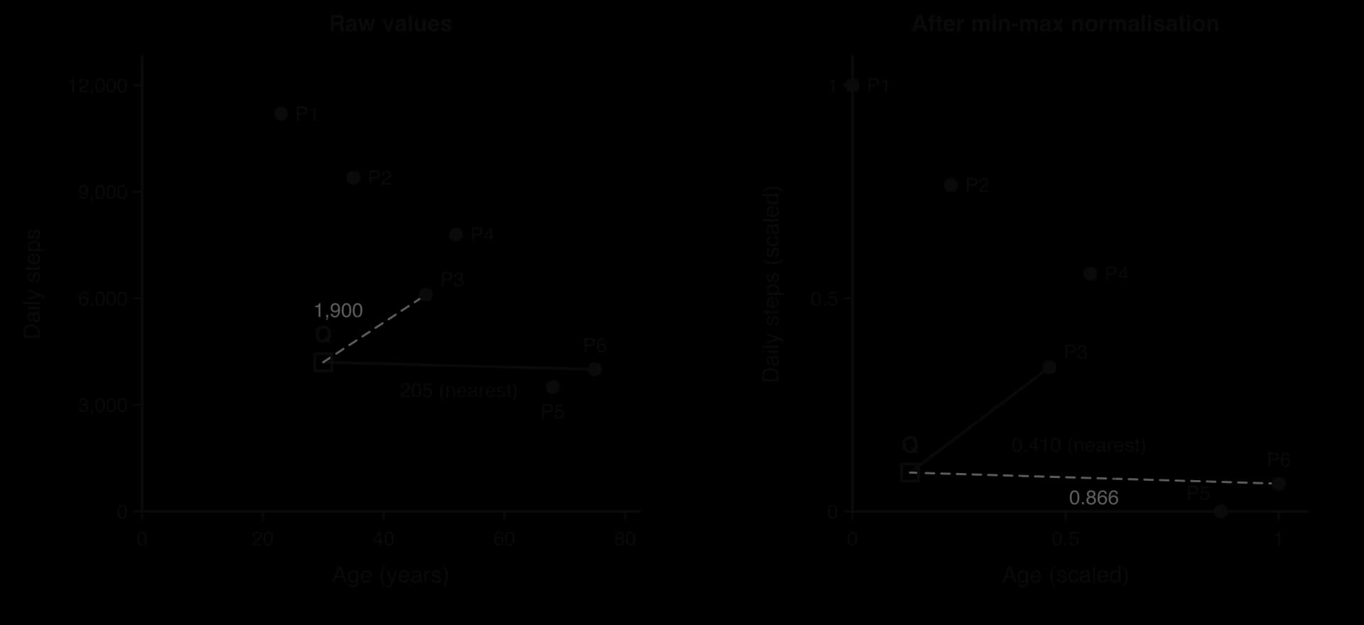
The hypothetical training set has six patients described by age and daily steps. A new patient Q is 30 years old and walks 4,200 steps a day.

Distances from the new patient Q before and after min-max normalisation (age range 23–75, step range 3,500–11,200, both from the training set). The nearest neighbour changes from P6 to P3.

On the raw values, Q's nearest neighbour is P6, a 75-year-old, because P6's step count is only 200 away; the 45-year age gap adds almost nothing to a distance of 205. After scaling, both features count equally and the nearest neighbour is P3, who is moderately close in both age and steps.

Scaling also matters for gradient-based algorithms such as artificial neural networks and linear regression trained step by step. These adjust each weight in proportion to the size of its feature's values, so with unscaled features some weights change in huge steps and others in tiny ones, and training takes far longer to settle or fails to settle at all. With scaled features, all the weights move at similar rates.

Not every algorithm needs scaling. A decision tree splits on one feature at a time with a threshold ("steps < 5,000?"), and scaling a feature moves the threshold but not the split, so trees give the same results with or without it.

Normalisation (min-max scaling)

Normalisation rescales a feature so that its smallest value becomes 0 and its largest becomes 1:

The minimum maps to 0, the maximum to 1, and every other value keeps its relative position between them. Normalisation suits features with known, natural bounds and few outliers. Image pixels are the standard case: each greyscale pixel in MNIST is stored as an unsigned byte from 0 to 255, so dividing every pixel by 255 normalises the image to the range 0 to 1.

Standardisation (z-score scaling)

Standardisation rescales a feature so that its mean becomes 0 and its standard deviation becomes 1, by replacing every value with its z-score:

A standardised value says how unusual the original value is for that feature: +1 means "one standard deviation above average", whatever the units were. This makes features with different units directly comparable. Standardisation suits features with no natural bounds and is the usual default for linear models and neural networks.

Choosing between normalisation and standardisation

Normalisation and standardisation compared. Both change the scale of a feature but not the shape of its distribution or the order of its values.

The effect of an outlier on min-max scaling is easy to see with numbers. If a seventh patient's step count were wrongly recorded as 40,000, the maximum would jump from 11,200 to 40,000. The six genuine patients, who previously spread across the whole range 0 to 1, would then all fall between 0 and 0.211, and the differences between them would almost vanish from any distance calculation. Standardisation is also affected, because the outlier raises both the mean and $\sigma$, so neither method replaces cleaning: outliers are dealt with first, and the scaling parameters are calculated afterwards.

Data leakage: fit on the training data only

The minimum, maximum, mean and standard deviation used for scaling are themselves learned from data. If they are calculated from the whole dataset before it is split, information about the test set (its largest value, its average) leaks into the training process. The test set is meant to stand in for future data the model has never seen, and future data cannot influence today's preprocessing, so the test score becomes slightly too optimistic.

The correct procedure is to split first, fit the scaler on the training set (calculate its parameters), and then apply the same parameters to the training set, the test set and every future input. Imputation follows the same rule: the median used to fill gaps in the test set is the median of the training set. The listing fits both scalers on the training step counts and applies them to two test values, one of which is outside the training range.

import math


def fit_min_max(train):
    low = train[0]
    high = train[0]
    for x in train:
        if x < low:
            low = x
        if x > high:
            high = x
    return low, high


def fit_standard(train):
    total = 0
    for x in train:
        total = total + x
    mean = total / len(train)
    squares = 0
    for x in train:
        squares = squares + (x - mean) ** 2
    return mean, math.sqrt(squares / len(train))


train_steps = [11200, 9400, 6100, 7800, 3500, 4000]
test_steps = [4200, 13500]

low, high = fit_min_max(train_steps)
mean, sd = fit_standard(train_steps)
print("min", low, , high, , mean, , (sd, ))
 x  test_steps:
    normalised = (x - low) / (high - low)
    standardised = (x - mean) / sd
    (x, (normalised, ), (standardised, ))

public class Scaling {
    static double[] fitMinMax(int[] train) {
        int low = train[0];
        int high = train[0];
        for (int x : train) {
            if (x < low) {
                low = x;
            }
            if (x > high) {
                high = x;
            }
        }
        return new double[] {low, high};
    }

    static [] fitStandard([] train) {
           ;
         ( x : train) {
            total = total + x;
        }
           total / train.length;
           ;
         ( x : train) {
            squares = squares + Math.pow(x - mean, );
        }
          [] {mean, Math.sqrt(squares / train.length)};
    }

       {
           Math.pow(, places);
         Math.round(value * factor) / factor;
    }

        {
        [] trainSteps = {, , , , , };
        [] testSteps = {, };

        [] range = fitMinMax(trainSteps);
        [] stats = fitStandard(trainSteps);
           range[], high = range[], mean = stats[], sd = stats[];
        System.out.println( + low +  + high +  + mean +  + round(sd, ));
         ( x : testSteps) {
               (x - low) / (high - low);
               (x - mean) / sd;
            System.out.println(x +  + round(normalised, ) +  + round(standardised, ));
        }
    }
}

min 3500 max 11200 mean 7000.0 sd 2771.9
4200 0.091 -1.01
13500 1.299 2.345

The Java version prints the same numbers, with 3500.0 and 11200.0 for the minimum and maximum because it stores them as double values. Java has no built-in method to round to a number of decimal places, so the listing defines its own round; Python's round(x, 3) does this directly. The test value 13,500 normalises to 1.299, above 1, because it is larger than any training value.

Feature selection

A dataset may have dozens, hundreds or thousands of features. Not all of them help: some are irrelevant, some repeat information that another feature already carries, and some are noise. Feature selection keeps the subset of existing features that is most informative for the task and discards the rest.

Fewer, better features bring several benefits:

• Less overfitting: with fewer features, there are fewer chance patterns for the model to memorise, so it generalises better to new data.

• Faster training and prediction: every feature removed is one less column to process for every record.

• Simpler, more interpretable models: a doctor can understand and check a model that uses five measurements far more easily than one that uses 500.

• Cheaper data collection: a feature that is not needed does not have to be measured, stored or protected in future.

• A weaker curse of dimensionality: fewer features keep the data denser and distances more meaningful.

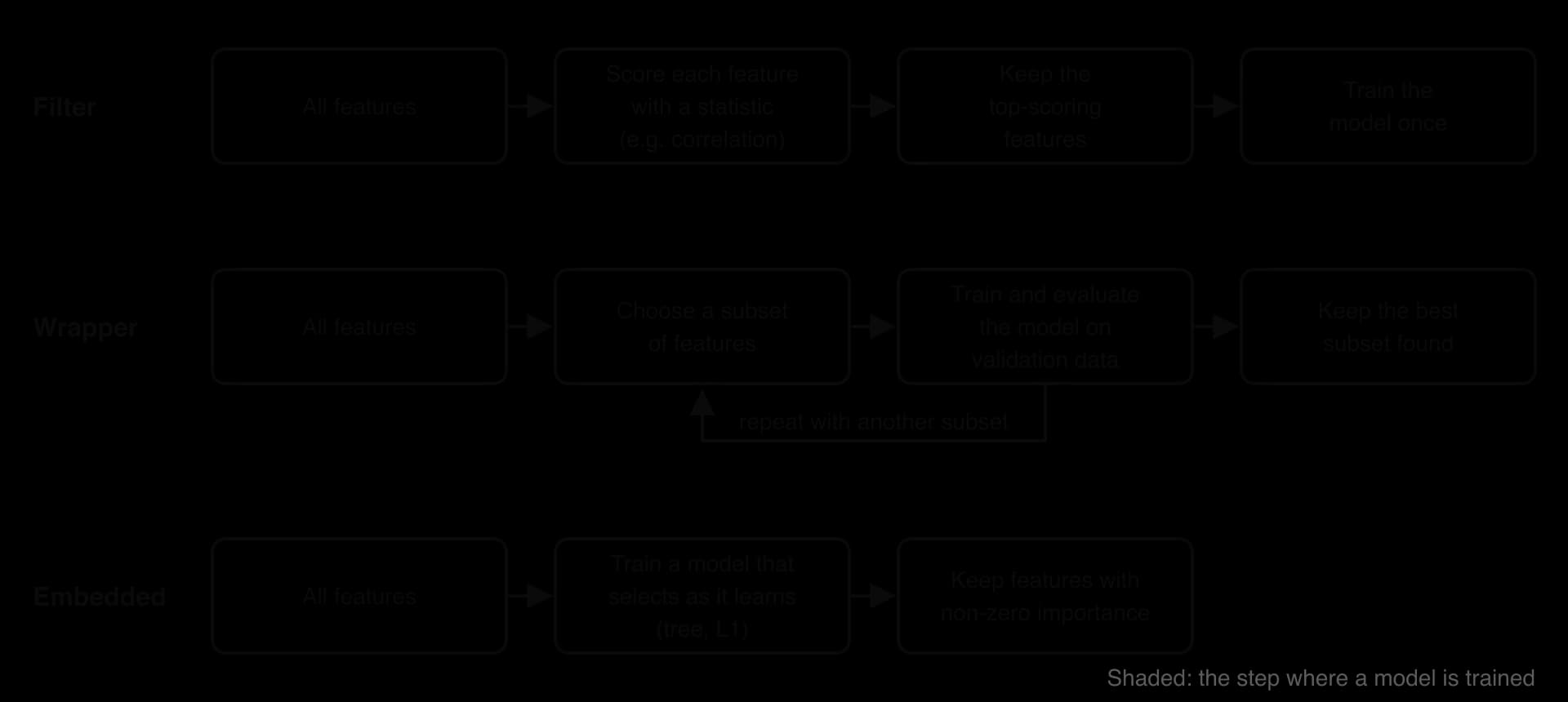
The methods fall into three families, which differ in whether, and how, they use a model to judge the features.

Filter methods

A filter method scores each feature with a statistic that measures its link with the target, independent of any model, and keeps the best-scoring features. Common statistics are:

• the correlation coefficient $r$ between a numeric feature and a numeric target (values near +1 or −1 mean a strong linear link; near 0 means none);

• the variance of the feature: a feature that is nearly constant (99% of records have the same value) cannot distinguish one record from another;

• a chi-squared test for categorical features against a categorical target;

• mutual information, which measures how much knowing the feature reduces uncertainty about the target, including non-linear links.

Filters are quick to run, because each feature is scored once, and they work the same whatever model is used afterwards. Their weakness is that each feature is judged on its own. A filter cannot see that two features are useful only in combination, and it cannot see that two highly ranked features carry the same information. Redundancy is handled by an extra step: if two selected features are strongly correlated with each other, only one is kept.

A hypothetical teacher has data on eight students and wants to predict their test score. The features are hours studied per week, practice papers completed, hours of sleep per night, student ID number and shoe size (EU). The correlation coefficient of each feature with the test score, calculated from the eight records, is:

The weakness of judging features alone can be extreme. Suppose the target is 1 when exactly one of two binary features A and B is 1, and 0 otherwise, the XOR pattern from subtopic A1.2, Data representation and computer logic. With the four records (0, 0), (0, 1), (1, 0) and (1, 1), the correlation of A with the target is exactly 0, and so is the correlation of B. A filter discards both, yet together they predict the target perfectly.

Wrapper methods

A wrapper method "wraps" the feature search around a real model. It tries different subsets of features, trains the chosen model on each subset, measures how well it performs on validation data, and keeps the subset that performs best.

Trying every possible subset is impossible for more than a few features: with $p$ features there are $2^p - 1$ non-empty subsets, over a million for $p = 20$. Wrappers therefore search greedily:

1. Forward selection starts with no features. In each round it tries adding each remaining feature, keeps the one that improves performance most, and stops when no addition helps.

2. Backward elimination starts with all the features. In each round it tries removing each one, removes the feature whose loss hurts least (or helps), and stops when every removal makes the model worse.

3. Recursive feature elimination trains the model on all features, removes the feature the model ranks as least important, and repeats until the desired number remains.

A hypothetical model predicts readmission from four features: age (A), blood pressure (B), number of previous admissions (C) and daily steps (D). Forward selection is used, and each candidate subset is scored by its accuracy on validation data:

Wrappers usually find a better subset for the chosen model than filters do, because they test features in combination and with the actual model. Their costs are time (each candidate subset means training a model, which is very slow for large datasets or models) and a risk of overfitting the feature choice itself: after hundreds of trials, the "best" subset may simply be the one that happened to suit the validation data. A subset chosen for one model may also not suit a different model.

Embedded methods

An embedded method selects features as a natural part of training the model, so no separate search is needed.

Two examples show the idea. A decision tree chooses, at every split, the feature that best separates the classes, so features that never help are never used; the total improvement each feature brings across all its splits gives its feature importance. L1 regularisation (also called Lasso) adds a penalty to a linear model in proportion to the total size of its weights (the sum of their absolute values); during training, the weights of features that add little are pushed to exactly zero, which removes those features from the model.

The three families of feature selection methods compared.

Feature selection and feature extraction

Feature selection chooses among the existing features. Feature extraction creates new features from the existing ones. Body mass index (BMI), calculated as mass divided by height squared, replaces two features with one that often predicts health outcomes better than either alone. Converting a date of birth into an age, or a timestamp into "day of the week", are also feature extraction.

The curse of dimensionality

Dimensionality

Each feature of a dataset is one dimension: a record with two features is a point on a plane, a record with three features is a point in 3D space, and a record with 784 features is a point in a 784-dimensional space that cannot be drawn but follows the same mathematics.

High dimensionality is common. Each MNIST image of a handwritten digit is 28 × 28 pixels, so each image is a record with 784 features, one per pixel. A text document represented by which of 50,000 dictionary words it contains has 50,000 features. One-hot encoding a field with 200 categories (countries, for example) adds 200 features at once.

Data sparsity and sample size

Space grows very fast as dimensions are added. Dividing each feature's range into 5 intervals gives 5 cells in one dimension, $5^2 = 25$ cells in two, and $5^3 = 125$ in three. Ten records fill all 5 cells of the line, at most 10 of the 25 cells of the square (40%), and at most 10 of the 125 cells of the cube (8%). The records are the same in each case, yet they become sparse, with most of the space holding no data at all.

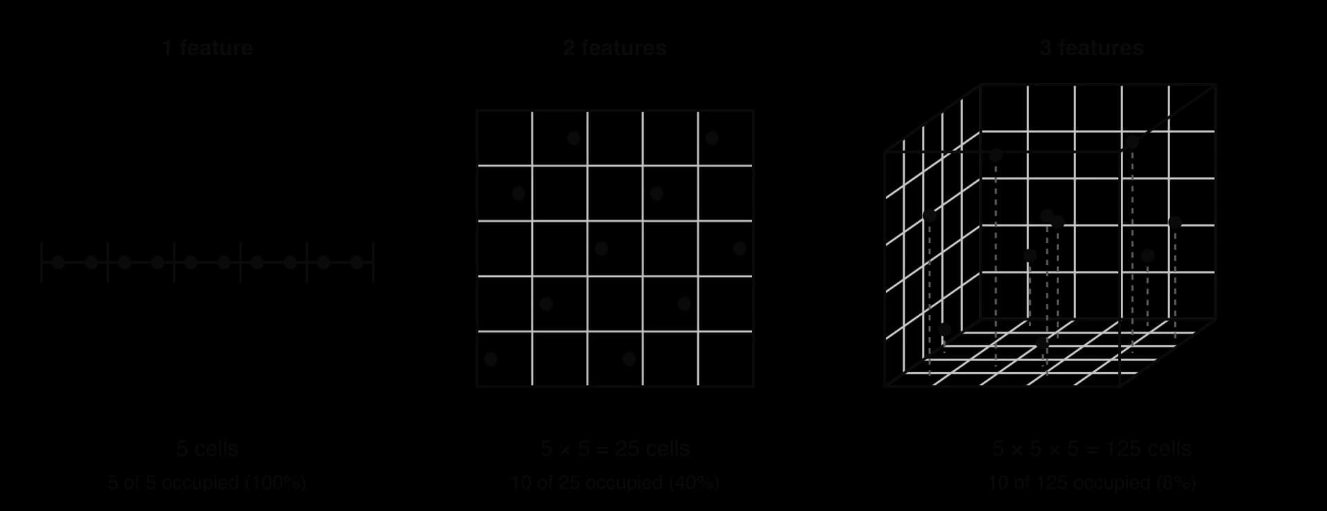
Sparsity explains why high-dimensional data needs far more records. To keep the same density, say 2 records per cell, the number of records must grow as fast as the number of cells: 10 records in one dimension, 50 in two, 250 in three, and with 10 features $2 \times 5^{10} = 19{,}531{,}250$. In practice no dataset grows that fast, so as features are added the data becomes thinner and the model must guess about more and more of the space. The required sample size grows exponentially with the number of features.

A second calculation shows the same effect from another angle. Suppose a model looks for the training records "near" a new input by taking a small cube around it that contains 10% of the data. In one dimension the cube's side covers 10% of each feature's range. In $d$ dimensions its side must cover $0.1^{1/d}$ of each range, because its volume is the side length to the power $d$.

Distance metrics lose their meaning

Many algorithms rely on a distance metric to decide which records are similar: k-NN finds the nearest training records, k-means assigns each record to the nearest cluster centre, and anomaly detection flags records that are far from all others.

In high dimensions this assumption breaks down. Each new feature adds its own small random difference to every distance, so all distances grow, and they grow together: the nearest and the farthest records end up at almost the same distance. When the nearest neighbour is hardly nearer than the farthest, "nearest" stops meaning "most similar". This is called distance concentration.

The program measures the effect. For each number of dimensions $d$, it places one query point and 500 other points at random in a cube with sides of length 1, and prints the distance to the nearest and farthest point and the ratio between them. The random numbers come from a simple formula (a linear congruential generator), written out so that the Python and Java versions produce identical numbers; the Python version uses the keyword global because the function changes the module-level variable seed.

import math

seed = 2027


def next_random():
    # A simple linear congruential generator, so Python and Java give the same numbers
    global seed
    seed = (seed * 1103515245 + 12345) % 2147483648
    return seed / 2147483648


def random_point(dimensions):
    point = []
    for i in range(dimensions):
        point.append(next_random())
    return point


def euclidean(a, b):
    total = 0.0
    for i in range(len(a)):
        total = total + (a[i] - b[i]) ** 2
    return math.sqrt(total)


print("    d  nearest farthest    ratio")
for d in [1, , , , ]:
    query = random_point(d)
    nearest = math.inf
    farthest = 
     n  ():
        distance = euclidean(query, random_point(d))
         distance < nearest:
            nearest = distance
         distance > farthest:
            farthest = distance
    ratio = farthest / nearest
    ()

public class Distances {
    static long seed = 2027;

    // A simple linear congruential generator, so Java and Python give the same numbers
    static double nextRandom() {
        seed = (seed * 1103515245L + 12345L) % 2147483648L;
        return seed / 2147483648.0;
    }

    static double[] randomPoint(int dimensions) {
        double[] point = new [dimensions];
         (   ; i < dimensions; i++) {
            point[i] = nextRandom();
        }
         point;
    }

       {
           ;
         (   ; i < a.length; i++) {
            total = total + Math.pow(a[i] - b[i], );
        }
         Math.sqrt(total);
    }

        {
        [] dims = {, , , , };
        System.out.println();
         ( d : dims) {
            [] query = randomPoint(d);
               Double.POSITIVE_INFINITY;
               ;
             (   ; n < ; n++) {
                   euclidean(query, randomPoint(d));
                 (distance < nearest) {
                    nearest = distance;
                }
                 (distance > farthest) {
                    farthest = distance;
                }
            }
               farthest / nearest;
            System.out.println(String.format(, d, nearest, farthest, ratio));
        }
    }
}

    d  nearest farthest    ratio
    1    0.001    0.603   535.85
    2    0.016    1.141    72.14
   10    0.481    1.840     3.83
  100    3.429    4.710     1.37
 1000   12.080   13.489     1.12

Both versions print this table. In one dimension the farthest point is over 500 times as far away as the nearest; with 1,000 features it is only 1.12 times as far, so every point is at roughly the same distance from the query. The Java seed is a long because the product seed * 1103515245 is far too large for an int; Python integers have no size limit, so no special type is needed.

YouTube

Overfitting, computation, memory and visualisation

Overfitting. Each feature gives a model more freedom to fit the training data. With many features and few records, a model can usually find some combination of features that separates the training examples perfectly, even if every feature is pure noise. It then memorises the training set instead of learning a general pattern, and performs poorly on new data. A model with 784 features trained on 200 images is almost certain to overfit.

Computational complexity. Most algorithms do work in proportion to the number of features for every record they process. A k-NN classifier for MNIST compares each test image with all 60,000 training images, and each comparison involves 784 pixel differences. Halving the number of features roughly halves this work.

Memory usage. The 70,000 MNIST images stored as one byte per pixel take $70{,}000 \times 784 = 54{,}880{,}000$ bytes, about 55 MB. Converted to 8-byte floating-point numbers for training, as most ML software does, they take about 439 MB. Datasets with millions of records and thousands of features quickly exceed the memory of a single computer.

Visualisation. People can see patterns in two or three dimensions only. A dataset with 784 features cannot be plotted directly, so clusters, outliers and mistakes in it are much harder to notice.

Dimensionality reduction

Dimensionality reduction lowers the number of features while keeping as much of the information relevant to the task as possible. It is the response to the curse of dimensionality: fewer dimensions mean denser data, more meaningful distances, less overfitting, less computation and memory, and, at two or three dimensions, a dataset that can be plotted.

The approaches divide into two kinds. Selection keeps some of the original features unchanged; extraction builds fewer new features from the old ones.

Ways of reducing the number of features. Each keeps the information most relevant to the task and discards detail that adds little.

Every reduction loses some information, so the aim is to lose the least useful part. Down-sampling MNIST to 14 × 14 keeps the shape of each digit but loses fine detail of the strokes; combining mass and height into BMI loses the difference between a short, light person and a tall, heavy one with the same BMI. Whether that loss matters depends on the task, which is why reduced datasets are checked by training a model and comparing its performance on validation data with the full dataset's.

Case study: the Netflix Prize data

The Netflix Prize was an open competition, launched by the film-rental company Netflix in October 2006, that offered US$1,000,000 to any team able to predict customers' film ratings 10% more accurately than Netflix's own system. The training data it released is one of the clearest real examples of sparse, high-dimensional data with most values missing.

Source: Netflix Prize (Wikipedia, citing Bennett and Lanning, 2007). The last three rows are calculated from the first three.

Sparsity. Arranged as a table with one row per user and one column per film, the data has 17,770 features per user, and 98.8% of the cells are empty. Two users have rated very few films in common, so measuring how similar they are rests on a small number of shared ratings. The distribution is also very uneven: the average user rated about 209 films, but some films in the training set had as few as 3 ratings, so any estimate about those films rests on almost no evidence.

Missing data that is not random. A rating is missing because a customer did not choose to watch and rate that film, and people mostly watch films they expect to like. The missing ratings are therefore likely to be lower, on average, than the recorded ones. Deleting incomplete rows is impossible (every user has gaps), and filling every gap with the film's mean rating erases the differences between users that the competition was about. Predicting the missing ratings from the known ones is predictive imputation on a vast scale, and it is the task the competitors were set; how the winning methods did it is covered in subtopic A4.3, Machine learning approaches.

Anonymisation as a preprocessing step. Before release, the data was prepared to protect customers. Users were given arbitrary ID numbers and no information about them was included, and some ratings were deliberately perturbed: a few were deleted, alternative ratings and dates were inserted, and some dates were changed. This preprocessing introduced a small amount of incorrect data on purpose, trading a little accuracy for privacy.

The preprocessing still did not make the records anonymous. Two researchers at the University of Texas at Austin, Arvind Narayanan and Vitaly Shmatikov, matched users' ratings of a few films against public reviews on the Internet Movie Database (IMDb) and identified some of them. The cause is the curse of dimensionality: with 17,770 film columns and an average of about 209 ratings per user, almost every user's sparse pattern of ratings is unique, so removing names does not remove identity, and small perturbations do not hide a pattern that distinctive.

Sources: "Netflix Prize", Wikipedia, accessed 2026; Narayanan and Shmatikov, "Robust De-anonymization of Large Sparse Datasets", IEEE Symposium on Security and Privacy, 2008.

The dataset brings several preprocessing themes together: missing data whose cause matters, a dimensionality so high that almost every record is unique, and a trade-off between keeping data accurate and altering it to protect the people it describes. The ethical side of that trade-off, including the privacy of people in training data, is developed in subtopic A4.4, Ethical considerations.

Exam focus

Data preprocessing is HL-only and is examined in Paper 1, Section A, usually as extra parts added to a machine learning question that SL students also answer. Questions on preprocessing mostly use describe, so most parts ask for a detailed account of a technique, its purpose and a consequence, for 2–4 marks each. Expect to describe two techniques for handling missing data or outliers in a given dataset, explain why features must be scaled before k-NN or k-means, calculate a normalised or standardised value, distinguish filter and wrapper methods, and describe problems caused by high dimensionality. Answers must be applied to the scenario in the question: name its features, its algorithm and its likely problems.

Command terms matter more than usual here, because many techniques can be described at very different depths. For describe, give the technique and how it works in the given dataset. An explain answer adds the reason ("because the distance is dominated by…"). In a calculate answer, show the substitution as well as the answer, and keep the training parameters fixed when a test value is involved.

Practice questions

1. Define the term outlier. [1]

2. State the formula for min-max normalisation and the range of the normalised training values. [2]

3. The values of a feature in a training set are 12, 15, 18, 20, 22, 25, 27 and 90. Calculate the lower and upper fences using the 1.5 × IQR rule and identify any outliers. [4]

4. A feature in the training data has mean 50 and standard deviation 8. Calculate the standardised value of 38 and of 70. [2]

5. Outline why one-hot encoding is used instead of numbering the categories 1, 2, 3 for a feature such as "favourite subject". [2]

6. A company has customer records merged from its website and its shops. Describe how near-duplicate records could be found and handled. [3]

7. Explain why calculating the mean for imputation on the whole dataset before splitting it into training and test sets is a problem. [3]

8. Describe one advantage and one disadvantage of an embedded method of feature selection compared with a filter method. [4]

9. A dataset has 8 features, each split into 4 intervals. Calculate the number of cells in the feature space and explain what this suggests about a dataset of 2,000 records. [3]

10. A hospital collects 600 features per patient but has records for only 400 patients. Discuss whether dimensionality reduction should be applied before training a model. [6]

Summary

• Data preprocessing turns raw data into a clean, consistent, numeric dataset. Because of "garbage in, garbage out", data quality limits a model's performance whatever the algorithm.

• Outliers are found with box plots, the 1.5 × IQR rule (fences at $Q_1 - 1.5 \times \text{IQR}$ and $Q_3 + 1.5 \times \text{IQR}$

Self-check

• To do:

  I can explain "garbage in, garbage out" and name the dimensions of data quality.

• To do:

  I can find the quartiles, IQR and fences for a small dataset and identify its outliers.

• To do:

  I can calculate a z-score and explain why the z-score rule can miss outliers in a small dataset.

• To do:

  I can decide whether to correct, remove, cap or keep an outlier, and justify the choice.

• To do:

  I can identify duplicate, incorrect, irrelevant, badly formatted and missing data in a table of records.

• To do:

  I can one-hot encode a categorical feature and explain why numbering categories is wrong.

• To do:

  I can compare deletion, mean, median and mode imputation, and predictive imputation, and choose one for a given feature.

• To do:

  I can calculate normalised and standardised values, including for a test value outside the training range.

• To do:

  I can explain, with a distance calculation, why k-NN needs scaled features.

• To do:

  I can explain data leakage and why scalers are fitted on the training data only.

• To do:

  I can distinguish filter, wrapper and embedded feature selection, with an example of each.

• To do:

  I can trace forward selection from a table of validation scores.