 YouTube
Describe how supervised, unsupervised, reinforcement, deep and transfer learning work, match them to real applications, and choose hardware from laptops to TPUs, edge devices, cloud platforms and supercomputers.
Each is in the Computer Science glossary, with every other term in the subject.
In reinforcement learning, the program that observes its environment, chooses actions and learns from the rewards those actions earn.
A chip designed and manufactured to perform one specific task, giving the highest speed and energy efficiency for that task but unable to be changed for other tasks.
The field of computer science that builds systems able to perform tasks normally thought to need human intelligence, such as recognising speech, making decisions or playing games.
A machine learning model made of layers of connected units (artificial neurons), in which each unit combines its weighted inputs and passes the result to the next layer; training adjusts the weights.
A supervised learning task in which the model predicts which of a fixed set of categories (classes) an input belongs to.
A service from a cloud provider that rents out machine learning hardware such as GPUs and TPUs on demand, together with storage and tools for training, deploying and monitoring models.
An unsupervised learning task that divides unlabelled examples into groups (clusters) so that examples in the same group are more similar to each other than to examples in other groups.
Describe the relationship between artificial intelligence, machine learning and deep learning.
Describe how a machine learning model is trained on a dataset and then used for inference, including the roles of features, labels, training data and test data.
Describe supervised, unsupervised and reinforcement learning, and the kind of data and feedback each one uses.
Describe deep learning and transfer learning, and how each relates to the other types of machine learning.
Identify the type of machine learning used in real-world applications, including market basket analysis, medical imaging diagnostics, natural language processing, object detection, robot navigation and sentiment analysis.
Describe the processing, storage and scalability requirements of machine learning, and how they differ between training and inference.
Describe the hardware used for machine learning, from standard laptops to GPUs, TPUs, ASICs, FPGAs, edge devices, cloud-based platforms and high-performance computing centres.
Describe a suitable hardware configuration for a given machine learning scenario, with reasons.
Machine learning is the part of computer science that builds programs which improve at a task by learning from data instead of following rules written by a programmer. A spam filter that has seen millions of emails marked "spam" or "not spam", a phone that recognises its owner's face and a translation service that turns Spanish into Korean all depend on it. Because a model is only as good as the data and the computing power behind it, the subject joins two questions: which kind of learning fits a problem, and which hardware can train and run the result at the required speed and cost.
90 exam-style questions on this subtopic, written in the style of the IB papers. The first has its markscheme open. Counted on
A hospital has 40 000 chest X-ray images. A radiologist has tagged each image as either pneumonia or healthy. The hospital wants a machine learning model that flags new X-rays that may show pneumonia.
Identify the type of machine learning the hospital should use.
1 mark
Supervised learning;
Note: Accept "supervised learning using deep learning". Do not accept "deep learning" alone.
Outline why the radiologist's tags are needed to train this model.
2 marks
Award [1] for the point and [1] for the development.
The tags are the labels / correct answers for each training image;
the model learns the link between image features and the label / compares its prediction with the tag and adjusts;
without labels the model would have no way of knowing which images show pneumonia;
so it could not learn to predict the category for new images;
Describe how the trained model would be used when a new patient's X-ray is taken.
One of 50 short multiple-choice questions on A4.1. Pick an answer to see why it's right or wrong.
A small firm fine-tunes a pre-trained image network to recognise four kinds of fabric fault. At first, which part of the network is trained?
The official deck for this part of the syllabus.
What is artificial intelligence (AI)?
State the two ways an AI system can get the rules it follows.
With a free account, Augment remembers where you stopped and what you have practiced.
A structured collection of examples used to train or test a machine learning model, where each example records the same set of properties.
Machine learning that uses artificial neural networks with many layers, which learn their own features in stages directly from raw data such as images, audio or text.
A device at the edge of a network, close to where data is produced, such as a phone, camera, sensor or car, that runs machine learning models locally instead of sending data to a remote server.
Everything outside the agent that it interacts with: it receives the agent's actions and responds with a new situation and a reward.
One measurable property of an example that is given to a machine learning model as an input, such as the number of links in an email or the floor area of a house.
A chip containing a large grid of logic blocks whose connections can be reconfigured after manufacture, so it can be programmed to act as a custom hardware circuit for a particular task and reprogrammed later.
Further training of a pre-trained model on a smaller, task-specific dataset, usually with a new output layer and small changes to the existing weights.
Floating-point operations per second, a measure of a processor's arithmetic speed; large values use prefixes such as tera (), peta () and exa ().
Machine learning models that produce new content, such as text, images, audio or code, resembling the data they were trained on.
The use of supercomputers, very large clusters of processors connected by fast networks and run as one system, to solve problems too large for ordinary computers.
The use of a trained model to produce an output, such as a prediction or classification, for new input data that the model has not seen before.
The known correct output attached to an example in a dataset, which a supervised learning model learns to predict from the features.
A very large deep learning model, pre-trained on huge amounts of text, that processes and generates human language by repeatedly predicting the next part of a text.
A branch of artificial intelligence in which a program improves its performance at a task by finding patterns in data, instead of following rules written explicitly by a programmer.
The analysis of customers' purchase records to find products that are frequently bought together.
The use of machine learning to analyse medical images, such as X-rays, scans or photographs of skin, to detect or classify signs of disease.
The result of training a machine learning algorithm on data: a stored set of learned values and structure that maps an input to an output, such as a prediction or a decision.
Techniques that reduce the size and computing needs of a trained model so it can run on limited hardware, such as storing weights with fewer bits (quantisation) or removing weights that contribute little (pruning).
The branch of AI that enables computers to analyse, understand and generate human language in text or speech.
The machine learning task of finding objects in an image or video, marking each one's position (usually with a bounding box) and classifying what it is.
A model that has already been trained on a large, general dataset and is made available for reuse as the starting point for other tasks.
A supervised learning task in which the model predicts a continuous numerical value, such as a price, a temperature or a score.
A type of machine learning in which an agent learns by trial and error which actions to take in an environment, by receiving rewards for good outcomes and penalties for bad ones.
A numerical signal that the environment gives an agent after an action, positive for desirable outcomes and negative (a penalty) for undesirable ones, which the agent learns to maximise over time.
The use of machine learning and sensor data to let a robot work out where it is and plan and control its movement through an environment towards a goal while avoiding obstacles.
The use of natural language processing to classify the opinion or emotion expressed in a piece of text, for example as positive, negative or neutral.
A type of machine learning in which a model is trained on labelled data, learning to map each example's features to its known correct output so that it can predict the output for new examples.
An application-specific integrated circuit designed by Google to accelerate the matrix calculations of neural networks, used for both training and inference.
The part of a labelled dataset kept back from training and used afterwards to measure how accurately the model performs on examples it has not seen.
The stage in which a machine learning algorithm repeatedly adjusts a model's internal values using example data, so that the model's outputs become more accurate.
The part of a labelled dataset used to train a machine learning model.
A machine learning approach in which a model trained for one task is reused as the starting point for a related task, so that the new task needs far less data and training time.
A type of machine learning in which a model is trained on unlabelled data and finds structure in it, such as groups of similar examples or items that occur together, without being given correct outputs.
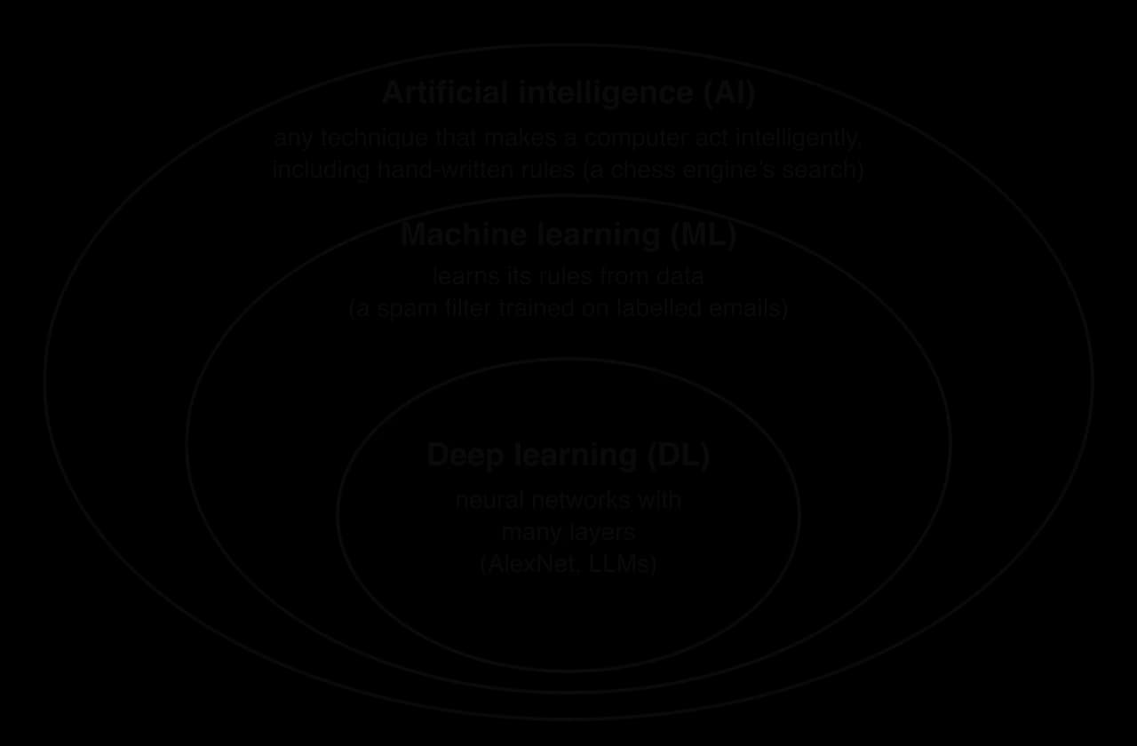
YouTubeThe three terms are often used as if they meant the same thing. They describe three nested ideas, each one a part of the one before it.
A chess program written in the 1990s that searches millions of possible moves and scores each position with a formula typed in by its programmers is AI, but it does not learn: its behaviour is fixed by the code. Machine learning takes a different route. Instead of writing the rules, the programmer writes an algorithm that finds the rules by studying examples.
The difference matters most for problems whose rules nobody can write down. No programmer can list the exact pixel patterns that make a photo show a cat, but a learning algorithm given many photos labelled "cat" and "not cat" can find patterns that separate them. Machine learning trades the effort of writing rules for the effort of collecting data, and the quality of the result depends on the quality of that data.
Deep learning is the part of machine learning that uses neural networks with many layers. The nested diagram shows how the three fields fit inside each other.
The result of machine learning is a model: a stored structure, often a large table of numbers, that turns an input into an output. A spam filter's model takes an email and outputs "spam" or "not spam"; a house-price model takes the size, location and age of a house and outputs a price.
A model passes through two stages in its life. During training, a learning algorithm adjusts the model's internal values again and again so that its outputs on known examples get closer to the right answers. Training is slow and heavy: a large model may need weeks of computation on thousands of processors. Once the values are fixed, the model is put to use, and each use is one inference: a single pass of a new input through the model to produce an output. One inference is usually quick, often milliseconds, but a popular service may run billions of them a day.
The split between the two stages shapes almost every decision about a machine learning system. It explains why a model can be trained once on a supercomputer and then copied to millions of phones, and why the hardware for training and the hardware for inference are often completely different.
Everything a model learns comes from its data. A dataset is organised much like a database table from subtopic A3.1: each row is one example (one email, one patient, one house) and each column records one property of it.
The columns that describe an example are its features, the inputs to the model. Choosing features is a form of abstraction: a house has thousands of properties, but a price model may use only five that matter. In supervised learning one column is special. It holds the right answer for each example, the label, which is the value the model must learn to predict.
The table shows part of a hypothetical dataset for a spam filter. Each row is an email, the first four columns are features and the last column is the label.
Links in email | Words in capitals | Sender in contacts | Contains "winner" | Label |
|---|---|---|---|---|
0 | 2 | Yes | No | not spam |
7 | 41 | No | Yes | spam |
1 | 0 | Yes | No | not spam |
5 | 18 | No | No | spam |
Labels are the expensive part of most datasets. Features can often be collected automatically (a server logs every email it receives), but someone has to decide whether each email is spam, whether each X-ray shows a tumour or whether each review is positive. Medical labels need specialists, so a labelled set of scans can cost far more than the scans themselves. This cost is one reason why unsupervised and transfer learning, which need few or no labels, are useful.
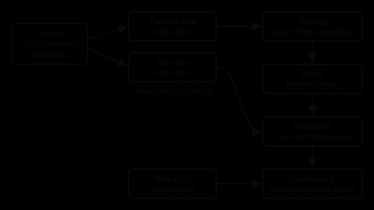
A model that has only been checked on the examples it learned from may simply have memorised them. To measure how well it will do on new inputs, the labelled dataset is split before training into two parts that never mix.
The larger part, commonly 70–80%, is used for training. The rest is kept aside and used only once training has finished, as a fair test of how the model behaves on examples it has never seen. A model that scores very well on its training data but poorly on its test data has learned details of those particular examples instead of the general pattern, a problem called overfitting.
The workflow diagram follows a labelled dataset of 10,000 examples from the split, through training and evaluation, to deployment.
The smallest possible example of training and inference fits in a few lines of code. The program spam_threshold learns one rule for a spam filter from twelve labelled emails, each with a single feature (the number of links). Training tries every threshold from 0 to 10, counts how many training emails the rule "spam if links ≥ threshold" gets wrong, and keeps the threshold with the fewest errors. That threshold is the whole model. The program then measures the model on five test emails and runs inference on two new ones.
# Training data: [number of links in an email, label]  (1 = spam, 0 = not spam)
training_data = [[0, 0], [1, 0], [2, 0], [3, 0], [4, 1], [2, 0],
                 [6, 1], [7, 1], [5, 1], [3, 1], [8, 1], [1, 0]]
test_data = [[0, 0], [5, 1], [2, 0], [6, 1], [4, 0]]


def count_errors(threshold, examples):
    errors = 0
    for example in examples:
        links = example[0]
        label = example[1]
        if links >= threshold:
            prediction = 1
        else:
            prediction = 0
        if prediction != label:
            errors = errors + 1
    return errors


def train(examples):
    # Try every threshold from 0 to 10 and keep the one with fewest errors
    best_threshold = 0
    best_errors = count_errors(0, examples)
    for threshold in range(1, 11):
        errors = count_errors(threshold, examples)
        if errors < best_errors:
            best_errors = errors
            best_threshold = threshold
    return best_threshold


def predict(threshold, links):
    if links >= threshold:
        return "spam"
    return "not spam"


model = train(training_data)
print("Learned rule: spam if links >=", model)
print("Training errors:", count_errors(model, training_data), "of 12")
print("Test errors:", count_errors(model, test_data), "of 5")
print("New email with 9 links:", predict(model, 9))
print("New email with 1 link:", predict(model, 1))public class SpamThreshold {
// Each row: {number of links in an email, label} (1 = spam, 0 = not spam)
static int[][] trainingData = {{0, 0}, {1, 0}, {2, 0}, {3, 0}, {4, 1}, {2, 0},
{6, 1}, {7, 1}, {5, 1}, {3, 1}, {8, 1}, {1, 0}};
static int[][] testData = {{0, 0}, {5, 1}, {2, 0}, {6, 1}, {4, 0}};
static int countErrors(int threshold, int[][] examples) {
int errors = 0;
for (int i = 0; i < examples.length; i++) {
int links = examples[i][0];
int label = examples[i][1];
int prediction;
if (links >= threshold) {
prediction = 1;
} else {
prediction = 0;
}
if (prediction != label) {
errors = errors + 1;
}
}
return errors;
}
static int train(int[][] examples) {
// Try every threshold from 0 to 10 and keep the one with fewest errors
int bestThreshold = 0;
int bestErrors = countErrors(0, examples);
for (int threshold = 1; threshold <= 10; threshold++) {
int errors = countErrors(threshold, examples);
if (errors < bestErrors) {
bestErrors = errors;
bestThreshold = threshold;
}
}
return bestThreshold;
}
static String predict(int threshold, int links) {
if (links >= threshold) {
return "spam";
}
return "not spam";
}
public static void main(String[] args) {
int model = train(trainingData);
System.out.println("Learned rule: spam if links >= " + model);
System.out.println("Training errors: " + countErrors(model, trainingData) + " of 12");
System.out.println("Test errors: " + countErrors(model, testData) + " of 5");
System.out.println("New email with 9 links: " + predict(model, 9));
System.out.println("New email with 1 link: " + predict(model, 1));
}
}Both versions print the same output.
Learned rule: spam if links >= 3
Training errors: 1 of 12
Test errors: 1 of 5
New email with 9 links: spam
New email with 1 link: not spam
The programmer never typed the rule "spam if links ≥ 3". The train subprogram found it by comparing eleven candidate rules against the labels. Thresholds 3 and 4 both make one training error (3 misclassifies the non-spam email with 3 links; 4 misclassifies the spam email with 3 links), and the strict < comparison keeps the first one found. The test email with 4 links that is not spam is misclassified, which shows that a rule fitted to training data is not perfect on new data. Real models differ in scale, with millions of values and features instead of one, but the stages are the same: learn values from labelled examples, measure on unseen examples, then run inference.
Machine learning approaches differ mainly in what feedback the learning algorithm receives. Supervised learning is told the right answer for every example; unsupervised learning is given no answers at all; reinforcement learning receives only a score for its actions, often long after it acted. Deep learning and transfer learning describe something else: the kind of model used, and where its starting knowledge comes from.
The three-panel diagram compares the three kinds of feedback.
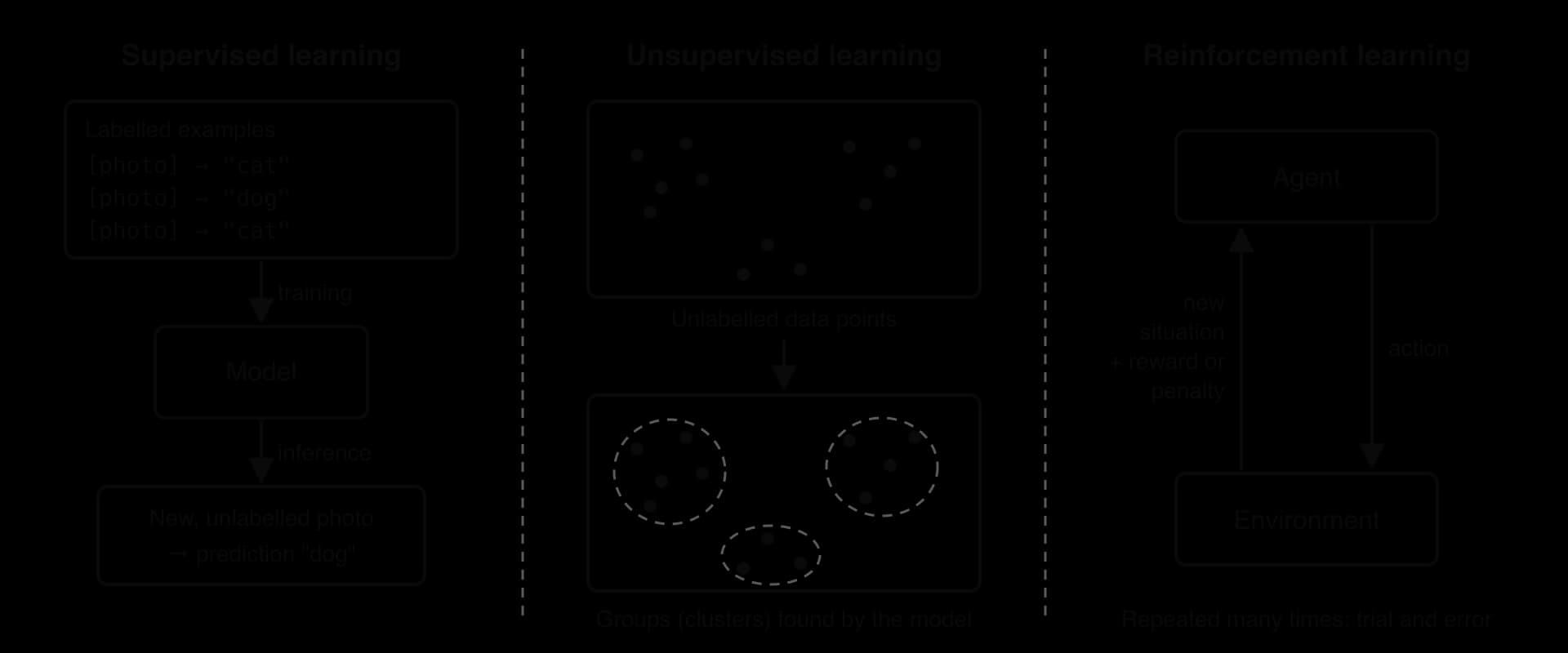
In supervised learning, every training example comes with its label, so the algorithm can compare its output with the right answer and adjust itself to reduce the difference. The name comes from this: the labels act like a teacher marking each answer.
Supervised learning solves two kinds of task, which differ in the type of output. When the output is one of a fixed set of categories, the task is classification. When the output is a number on a continuous scale, the task is regression.
A regression model draws a line or curve through the training examples and reads its prediction from it. The graph shows a hypothetical regression model that predicts a test score from hours of revision, fitted to eight students' results.
The same model also shows a limitation of supervised learning. Read at 20 hours, the line predicts a score of about 118, which is impossible on a 100-point test. A model is reliable only for inputs similar to its training data; outside that range (extrapolation) its predictions can be meaningless.
Supervised learning is the most widely used type because, when good labels exist, it gives a clear target and a clear way to measure success (the proportion of test examples predicted correctly). Its costs come from the labels. They may be expensive (each needs an expert), slow to gather, or wrong, and a model reproduces any errors and prejudices present in its labels, an issue of algorithmic bias. Typical algorithms, named here and explained only at HL, include linear regression, k-nearest neighbours and decision trees.
Many datasets have no labels: a supermarket's till receipts, the clicks on a website or the readings from a factory's sensors. Unsupervised learning looks for structure in such data without being told what to look for.
The most common unsupervised task is clustering. The algorithm measures how similar examples are, using their features, and places similar examples in the same group. Nobody tells it what the groups mean: a clustering of shoppers might produce one group that buys baby products and another that buys mainly ready meals, and a person then interprets the groups and names them.
A second task finds items that tend to occur together, known as association. A third, anomaly detection, finds examples that do not fit the usual pattern, such as a card payment unlike any the customer has made before. All three are also techniques of data mining. The algorithm explained at HL for clustering is k-means.
Unsupervised learning is cheap to feed, because unlabelled data is plentiful, and it can find patterns nobody thought to look for. Its weakness is evaluation: without labels there is no right answer to compare against, so a person must judge whether the clusters are useful, and the same data can be grouped in several equally defensible ways.
 YouTube
Some tasks are sequences of decisions in which no single move has a "correct" label: steering a robot through a warehouse, controlling a game character or adjusting a data centre's cooling. Reinforcement learning handles these by letting a program act, observe the outcome and receive a score.
The learner is called the agent. It observes its situation, chooses an action, and the environment responds: the situation changes and the agent receives a reward (a positive number) or a penalty (a negative one). Over many thousands or millions of attempts, the agent learns a strategy that collects as much reward as possible in total.
The environment can be a simulation (a game, a physics model of a robot arm) or the real world. Simulations are popular because an agent can try millions of actions quickly and safely there; a real robot that learns by falling over is slow and expensive.
Rewards are often delayed. In a board game, the only true reward may come at the end (a win or a loss), so the agent must work out which of its many earlier moves deserve the credit. This makes reinforcement learning slower and harder to train than supervised learning, and a badly designed reward can be exploited: an agent rewarded only for speed may learn to cut dangerous corners. Gerald Tesauro's TD-Gammon, developed at IBM in the 1990s, learned backgammon this way: it played about 1.5 million games against itself, using the result of each game as its reward, and, once given some hand-designed features as inputs, outplayed every earlier backgammon program.
The detailed vocabulary of reinforcement learning (states, policies, cumulative reward, and the balance between exploring new actions and exploiting known good ones) is HL content in subtopic A4.3.
Deep learning is built on artificial neural networks, which are loosely modelled on the way neurons in a brain pass signals to each other. A network is made of layers of simple units. Each unit takes numbers from the layer before, multiplies each by a weight, adds them up and passes the result on. Training adjusts the weights, of which a large network may have billions.
A network is "deep" when it has many layers between input and output. Depth lets the network build up its own features in stages. In an image network, the early layers learn to detect edges and colour changes, middle layers combine them into textures and shapes, and later layers combine those into parts of objects such as eyes or wheels. Earlier machine learning needed people to design features by hand (for example, "number of links" for spam); deep learning learns useful features directly from raw pixels, sound samples or text.
That ability has two costs. Deep networks need very large datasets, often millions of examples, because they have so many weights to set; and training them needs enormous numbers of arithmetic operations, which is why deep learning only became practical when graphics processing units (GPUs) were used to train it, as with AlexNet in 2012. Deep models are also hard to explain: a decision spread across millions of weights cannot be read like a rule, an issue for medicine and law covered in subtopic A4.4. The way individual neurons and convolutional neural networks work is HL content in subtopic A4.3.
Training a deep network from nothing needs millions of labelled examples and a large amount of computing. Most organisations have neither, but they can reuse a network someone else has already trained.
The insight behind transfer learning is that the early layers of a network trained on general images have learned features (edges, textures, simple shapes) that are useful for almost any image task. A hospital that wants to recognise skin cancer does not need to teach a new network what an edge is. It copies a network pre-trained on everyday photos, keeps its early layers, and replaces only the final layer with a new one for its own classes.
The new model is then trained briefly on the small task-specific dataset. Usually the copied layers are frozen (their weights are not changed) at first, and only the new layer learns; later, some copied layers may be unfrozen and adjusted slightly. The transfer learning diagram shows both stages.
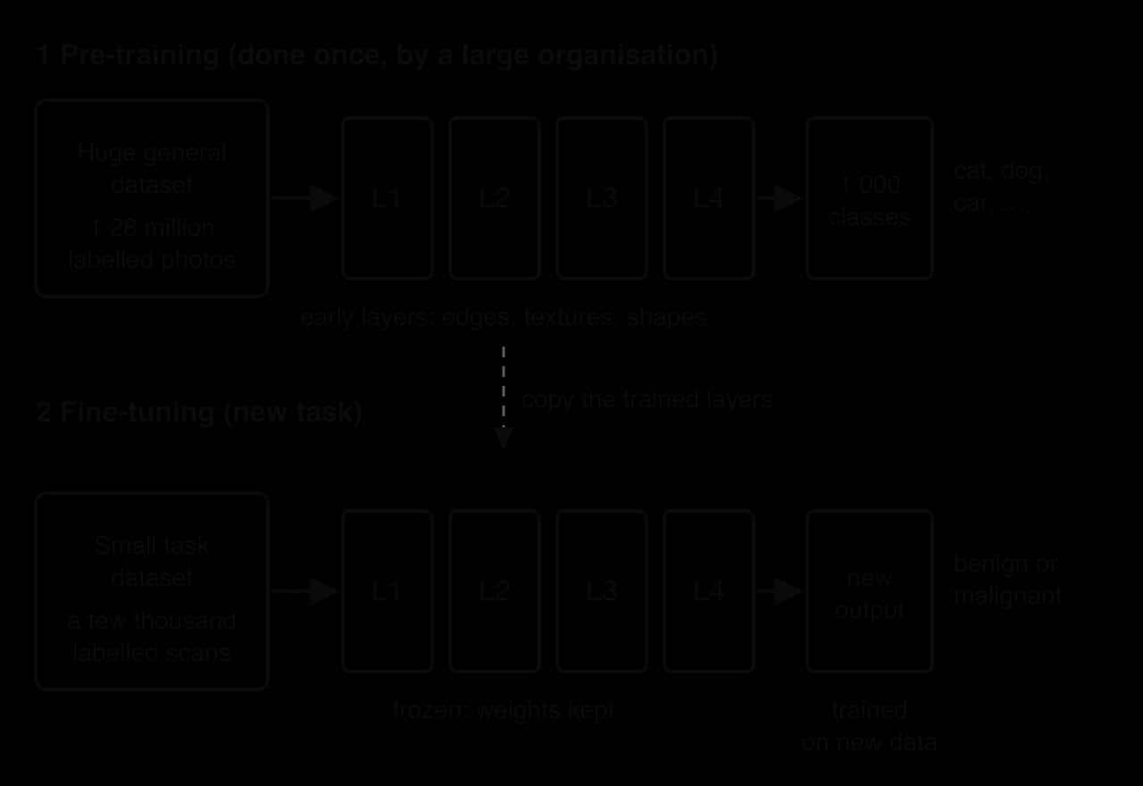
A well-known medical example comes from Stanford University in 2017. Researchers took Google's Inception v3 network, pre-trained on the 1.28 million images of the ImageNet challenge, and fine-tuned it on 129,450 clinical images covering 2,032 skin diseases. Tested against 21 board-certified dermatologists on biopsy-confirmed images, it performed on a par with all of them at telling cancers from harmless lesions. The same pattern underlies language technology: models such as Google's BERT (2018) are pre-trained once on huge amounts of text and then fine-tuned for tasks such as sentiment analysis.
Transfer learning saves data, time, money and energy, and it lets small organisations use deep learning at all. Its limits come from what the pre-trained model learned. If the new task is too different (a model pre-trained on everyday photos applied to radio telescope data), the copied features may not help. Any bias in the original training data is also carried into every model built on it, and users may not know what that data contained.
The table brings the five approaches together. The first three differ in the feedback they receive; the last two describe the model and how it is started.
Approach | How it learns | Data it needs | Typical tasks | Example application |
|---|---|---|---|---|
Supervised learning | Compares its outputs with known correct outputs | Labelled examples | Classification, regression | Sentiment analysis of labelled reviews |
Unsupervised learning | Finds structure in data with no correct outputs | Unlabelled examples | Clustering, association, anomaly detection | Market basket analysis |
Reinforcement learning | Acts, then receives rewards or penalties | An environment to act in (often a simulation) | Sequences of decisions | Robot navigation |
Deep learning | Many-layered neural network learns its own features | Very large datasets and heavy computation | Images, speech, text | Object detection |
Transfer learning | Reuses a pre-trained model, then fine-tunes it | A small task-specific dataset | Any task related to the original one | Medical imaging diagnostics |
Applications usually combine several approaches. The skill is to identify, for each one, what the input and output are, whether labelled data exists, and therefore which type of learning fits.
Shops record every basket of goods that passes through the tills. Market basket analysis searches these records for products bought together, such as pasta with a particular sauce, and the shop uses the results to place products, design offers and recommend items online.
It is unsupervised learning: no basket carries a label, and the algorithm finds association patterns ("customers who buy X often also buy Y") that nobody specified. How such rules are measured is HL content (association rules in subtopic A4.3).
Hospitals produce X-rays, CT and MRI scans, retinal photographs and microscope slides in large numbers. Models trained on scans labelled by specialists can flag likely tumours, fractures or eye disease, for a specialist to check first.
It is supervised deep learning, usually with transfer learning because labelled scans are scarce, as in the Stanford skin cancer model. The cost of an error is high, so these systems support clinicians instead of replacing them, and a model trained on one hospital's scanners or patient population may perform worse elsewhere.
Text and speech are the hardest data for rule-based programs, because human language is ambiguous and full of exceptions. Machine learning is now the main way computers handle it.
Modern NLP is dominated by deep learning and transfer learning. A very large network is pre-trained on huge amounts of text, learning to predict the next word, and is then fine-tuned for particular uses.
Pre-training on text needs no human labels, because the next word in each sentence acts as the label. Chat assistants add further supervised fine-tuning and reinforcement learning from people's ratings of answers. LLMs are an example of generative AI, which produces new content instead of only classifying existing content.
Companies want to know what customers think of a product, film or political issue, but reading millions of reviews and posts is impossible by hand. Sentiment analysis does it automatically.
It is a supervised classification task: the model learns from texts labelled with their sentiment (a review's star rating can serve as a ready-made label). Sarcasm ("Great, it broke on day two"), slang and mixed opinions remain difficult, and a model trained on film reviews may misread restaurant reviews.
Self-driving cars, security cameras, phone cameras and factory inspection systems need to know not only what is in an image, but where.
It is supervised deep learning, trained on images in which people have drawn boxes around objects and labelled them. In a car, detection runs many times per second on hardware inside the vehicle, so object detection is one of the main jobs given to edge devices.
A warehouse robot, a robot vacuum or a planetary rover must move through a space without hitting anything, often while the space changes around it.
Reinforcement learning suits it: the robot is the agent, the space is the environment, and it is rewarded for reaching its goal quickly and penalised for collisions. Training usually happens in simulation first. Real robots also use supervised deep learning to recognise what their cameras see, so one application combines two types.
The table summarises the six applications, the type of learning each typically uses and the data it needs.
Application | Main type of learning | Input → output |
|---|---|---|
Market basket analysis | Unsupervised (association) | Till receipts → products bought together |
Medical imaging diagnostics | Supervised deep learning, often transfer learning | Scan → disease or no disease |
Natural language processing | Deep learning and transfer learning (LLMs) | Text or speech → translation, answer, summary |
Sentiment analysis | Supervised (classification) | Review or post → positive, negative or neutral |
Object detection | Supervised deep learning | Image → boxes with labels |
Robot navigation | Reinforcement learning, plus supervised vision | Sensor readings → movement |
Hardware for machine learning is judged on three main factors, plus three that decide between otherwise suitable options.
Processing: how many arithmetic operations per second the hardware can perform. Neural networks are mostly multiplications and additions of large tables of numbers (matrices), so what matters is how many can run at the same time, through parallel processing.
Storage: the capacity and speed of memory and disks. The model's weights and a batch of training data must fit in the processor's fast memory (RAM, or the high-bandwidth memory on a GPU), and the dataset, from megabytes to petabytes, must be read from disks (SSDs or large disk arrays) fast enough to keep the processors busy.
Scalability: how easily more processing or storage can be added when the dataset or model grows, from one more GPU to thousands of machines working as a distributed system.
Power, cost and latency: energy use and heat, the price to buy or rent, and the delay between an input arriving and the output being ready.
Processing speed for machine learning is measured in operations per second, usually written in FLOPS.
The single biggest factor in choosing hardware is whether the system is training a model or running inference with it. Training processes the whole dataset many times (each full pass is an epoch) and must also store intermediate results to adjust every weight, so it needs the most processing and memory, but it can run for days in a data centre where nobody waits for an answer. Inference processes one input at a time and needs much less, but it often must answer within milliseconds, on a device with a battery, for millions of users at once.
Training | Inference | |
|---|---|---|
Work per run | The whole dataset, many passes | One input, one pass |
Memory | Weights, data batches and intermediate values | Mainly the weights |
Time scale | Hours to months | Milliseconds |
Typical hardware | GPU clusters, TPUs, HPC centres | Phones, edge devices, servers, cloud |
Main concern | Total processing power and scalability | Latency, energy and cost per inference |
An ordinary laptop's central processing unit (CPU) has a few fast cores designed for varied, sequential work with many branches. That is enough for learning machine learning, for prototyping, for classic algorithms on small datasets (thousands to a few million rows that fit in RAM), and for running inference with small or compressed models. Many laptops now also contain a modest GPU or a built-in neural accelerator.
The limits appear quickly with deep learning. A CPU performs relatively few multiplications at once, so training a large network could take months instead of days; its RAM is far too small to hold a large model and its training data; and a laptop cannot scale beyond the one machine. A laptop is a sensible choice when the dataset is small, the model is simple, or the work is a first experiment before moving to bigger hardware.
A GPU, described in subtopic A1.1, has thousands of simple cores that all apply the same operation to different numbers at the same moment. It was designed to calculate millions of pixel colours at once, and the matrix multiplications at the heart of neural networks have the same shape: large numbers of independent multiply-and-add operations. On this kind of work a GPU is many times faster than a CPU, and on sequential, branching work it is slower.
GPUs are the default hardware for training deep learning models. A single high-end GPU in a workstation can fine-tune a pre-trained model or train a medium-sized network; servers hold eight GPUs joined by fast links, and large models are trained on thousands of them at once. Their weaknesses are power consumption (hundreds of watts each), price, and limited on-board memory, which forces large models to be split across several GPUs.
 YouTube
A GPU is still a general-purpose parallel processor: it carries circuitry for graphics and for many kinds of calculation. A chip designed for one job only can leave all that out and spend its whole area and power budget on that job.
ASICs give the best performance per watt for their task, which matters both in data centres (where electricity is a large share of cost) and in battery-powered devices. Against this, designing a new chip costs a very large amount and takes years, so ASICs are worthwhile only for tasks performed on an enormous scale; and the function is fixed in the silicon, so if machine learning methods change, the chip cannot follow.
The best-known machine learning ASIC is Google's tensor processing unit. Google used the first TPUs internally from 2015, announced them in May 2016, and made them available to other companies through Google Cloud in 2018. The first version was an 8-bit matrix multiplication engine built around a 256 × 256 grid of multipliers, drawing 28–40 W, and it ran inference only. From the second version, announced in 2017, TPUs also handle training.
TPUs give high throughput and energy efficiency for training and serving large neural networks, and they can be connected in "pods" of many chips. Most organisations cannot buy data-centre TPUs; they rent them through Google Cloud, so choosing TPUs also means depending on one provider.
Between a fixed ASIC and a general-purpose processor sits a chip whose circuits can be rewired after manufacture.
An FPGA programmed as a circuit for one model runs it with very low and predictable latency, and with better performance per watt than a CPU or GPU, though usually below an ASIC. When the model changes, the FPGA is simply reprogrammed. Microsoft's Project Catapult placed FPGAs in its data centres, first to speed up the Bing search engine and later to run neural networks for its Azure cloud services. FPGAs are also used where reactions must be immediate, as in telecommunications and financial trading. Their drawbacks are the specialist skill needed to program them and a lower peak speed than a GPU for training, so they are used mainly for inference.
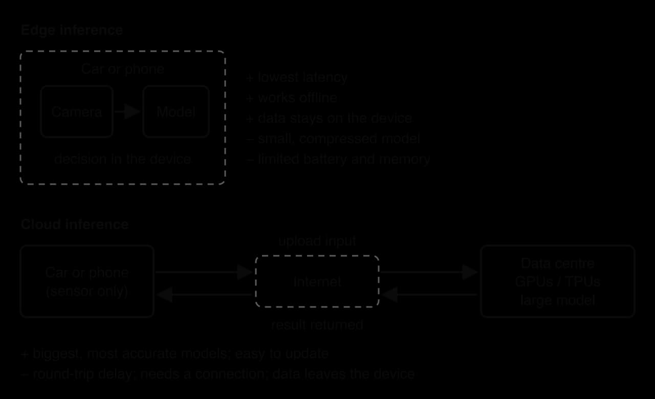
Sending every camera frame or voice recording to a distant data centre and waiting for an answer is too slow for some tasks, needs a constant connection, and sends private data away from its owner. Edge computing moves the processing to where the data is produced.
Edge devices nearly always run inference only: training happens in a data centre and the finished model is copied to the device. Their hardware is constrained (a battery, a few gigabytes of memory, no fans), so they use small ASICs and accelerators. Apple's A11 chip (iPhone X, 2017) included a Neural Engine able to perform up to 600 billion operations per second, used for Face ID, so the face never had to leave the phone. Google's Edge TPU, available to developers from 2019, performs 4 trillion operations per second using 2 W of power and supports only inference.
To fit a model on such hardware, developers shrink it.
The edge-versus-cloud diagram compares the two places where inference can run.
Many organisations need large amounts of GPU or TPU power only occasionally, while training a model. Cloud computing lets them rent it.
Renting is a form of infrastructure as a service: the provider owns, powers and maintains the machines. The main advantage is elastic scalability, the ability to rent eight GPUs this afternoon and a thousand next month, and release them when the job ends. There is no upfront purchase, the latest hardware is available as soon as the provider installs it, and the trained model can be deployed for inference on the same platform.
The disadvantages grow with use. Costs continue for as long as the hardware is rented, and a team that trains every week may pay more than buying its own GPUs; very large datasets are slow and expensive to upload; sensitive data such as medical records leaves the organisation's premises, raising privacy and legal questions; and moving to another provider can be hard once tools and data are in one cloud.
Some scientific simulations and very large training runs need thousands of processors working closely together on one problem for weeks.
What sets an HPC centre apart is its interconnect, a network fast enough for thousands of nodes to exchange results while working on one problem together. Frontier, at Oak Ridge National Laboratory in the United States, became the world's first exascale supercomputer in 2022, reaching 1.102 exaFLOPS ( operations per second) with AMD CPUs and GPUs. Such systems train scientific models (climate, materials, drug discovery) and very large neural networks. The costs are on the same scale: Frontier cost about US$600 million to build and draws around 21 megawatts of power, so HPC time is shared among many research projects and must be applied for.
The right configuration depends on the size of the dataset and the model, the number of users, and how fast or private the answers must be. The spectrum table compares the options on these factors.
Configuration | Processing | Storage | Scalability | Power and cost | Latency | Typical scenario |
|---|---|---|---|---|---|---|
Standard laptop | A few general-purpose CPU cores, perhaps a small GPU or neural accelerator | The laptop's own RAM and SSD | None beyond the one machine | Low power; usually already owned | Low for small local models | Learning, prototyping, small datasets |
GPU workstation or server | One to several GPUs | Dedicated GPU memory and fast SSDs | Limited to the slots in one box | High purchase price; each GPU draws far more power than a CPU | Low on site | Training medium models, fine-tuning |
Edge device | Small ASIC or NPU | Small memory, shared with the rest of the device | Scales by adding devices, each working alone | Very low power; cheap per unit | Lowest: no network round trip | Inference in phones, cameras, cars |
FPGA | Custom reprogrammable circuit | Memory on the board | Add more boards | Efficient, but needs specialist skill | Very low and predictable | Real-time inference with models that change |
Cloud GPUs and TPUs | Large pools of accelerators to rent | Elastic cloud storage | Elastic: up and down on demand | No upfront cost; pay for the hours used | Includes the network round trip | Training large models; serving many users |
HPC centre | Thousands of nodes of CPUs and GPUs with a fast interconnect | Very large parallel file systems | Very high, but shared among projects | Very high building and running costs | Batch jobs, not live answers | Huge models, scientific ML |
For training, capability rises from the laptop through the GPU server and the cloud to the HPC centre, and so does the cost. Edge devices and FPGAs sit apart from that line, because they are built to run inference quickly and cheaply rather than to train. Real products show how wide the range is. The product table gives published figures for one named example of most categories, spanning the GPUs that trained AlexNet, a phone's neural engine and the first exascale supercomputer.
Product (year) | Kind of hardware | Arithmetic speed | Memory | Power | Price or cost |
|---|---|---|---|---|---|
Nvidia GeForce GTX 580 (2010) | Consumer GPU (two trained AlexNet) | 1.581 TFLOPS (32-bit) | 3 GB in the version AlexNet used | – | About US$500 at release |
Apple A11 Neural Engine (2017) | ASIC inside a phone (edge device) | Up to 600 billion operations per second | Shares the iPhone X's 3 GB | – | – |
Google Edge TPU (2019) | Edge ASIC, inference only | 4 trillion operations per second | – | 2 W | – |
Google TPU, first version (2015) | Data-centre ASIC | 256 × 256 grid of 8-bit multipliers | 8 GiB | 28–40 W | Not sold |
Nvidia H100 SXM (2022) | Data-centre GPU | – | Up to 80 GB of high-bandwidth memory | 700 W | Estimated US$25,000–30,000 (2024) |
Frontier supercomputer (2022) | HPC centre: 9,472 CPUs and 37,888 GPUs | 1.102 exaFLOPS | 700 PB file system | About 21 MW | About US$600 million |
Sources: Wikipedia articles "AlexNet", "Apple A11", "Tensor Processing Unit", "Hopper (microarchitecture)" and "Frontier (supercomputer)", 2026; Coral (Google), "Edge TPU performance benchmarks", 2026. A dash means no comparable published figure.
Every option also has an environmental cost. Training large models uses large amounts of electricity, and accelerators are replaced every few years as faster ones appear. These issues of environmental impact and electronic waste are discussed in subtopic A4.4.
AlexNet is the deep learning model that showed, in 2012, that deep neural networks trained on GPUs could beat every other approach to recognising images. It combines supervised deep learning, a large labelled dataset and hardware chosen to make training possible.
AlexNet was built by Alex Krizhevsky, with Ilya Sutskever and Geoffrey Hinton, at the University of Toronto, and entered in the ImageNet Large Scale Visual Recognition Challenge. The challenge gave teams about 1.2 million training photos, each labelled with one of 1,000 categories, and scored each model on new images. A model's answer counted as correct if the right category was among its five most likely guesses; the proportion it got wrong is its top-5 error.
Feature | AlexNet (2012) |
|---|---|
Type of learning | Supervised deep learning (image classification) |
Training data | About 1.2 million labelled images, 1,000 classes |
Size of model | About 60 million weights |
Hardware | Two Nvidia GTX 580 GPUs, 3 GB of memory each |
Training time | 90 passes over the data (epochs) in five to six days |
Result | 15.3% top-5 error, more than 10.8 percentage points better than the runner-up |
Source: Krizhevsky, Sutskever and Hinton (2012), as summarised in Wikipedia, “AlexNet”, 2026.
The winning margin came from depth. Earlier entries relied on features designed by researchers; AlexNet's eight layers learned their own features from the raw pixels, from edges in the first layer to object parts in the last. That needed both the 1.2 million labelled images, which had become available only with ImageNet, and far more computation than earlier models. Its success made supervised deep learning the standard method for object detection and medical imaging, and AlexNet-style networks pre-trained on ImageNet became the most common starting point for transfer learning. Its internal design (convolutional and pooling layers) is studied at HL in subtopic A4.3.
The training workload was more than a billion arithmetic operations per image, most of them independent multiplications, repeated over 1.2 million images 90 times:
The work in each of those 108 million passes was mostly independent multiplications, an ideal job for parallel processing. Two consumer graphics cards, sold for gaming at about US$500 each, did it in under a week, where CPUs of the time would have taken far longer. The case also shows the storage limit that still shapes ML hardware: the network did not fit in the 3 GB memory of one GPU, so the team split it into two halves, one per GPU, exchanging results only at certain layers. Today's models are split across thousands of GPUs for the same reason, which is why GPU memory size, fast links between GPUs and scalable cloud and HPC systems matter as much as raw speed.
AlexNet's success came from three factors arriving together: a large labelled dataset, an algorithm that could use it, and affordable parallel hardware, and none of the three would have been enough without the other two. The table sets out what each factor contributed and the general lesson for choosing ML systems.
Factor | In AlexNet | General lesson |
|---|---|---|
Data | 1.2 million labelled ImageNet images | Deep models need very large labelled datasets, or transfer learning |
Model | Eight layers that learned their own features | Depth replaces hand-designed features but multiplies the computation |
Hardware | Two consumer GPUs working in parallel | Parallel processors and enough memory decide what can be trained at all |
The same reasoning applies to choosing hardware for any ML scenario: the size of the data and the model sets the processing and storage needed. This pattern of ever larger data and models also drove a sharp rise in the energy and money spent on training ever larger models, and a dependence on a small number of GPU makers, issues taken up in subtopic A4.4.
Machine learning fundamentals is examined in Paper 1 Section A, at both SL and HL, and often in Section B when the case study involves an ML system. Both content statements use Describe (AO2), so questions ask for detailed accounts: the features of a type of learning, how an application uses it, or what hardware a scenario needs. Closely related terms appear as Identify (which type of learning or which hardware fits a scenario, 1–2 marks), Outline (a brief account, 2 marks) and Distinguish (supervised versus unsupervised). Applying the ideas to an unfamiliar scenario is where most marks are won and lost; a scenario's details (no labels available, no network connection, a limited budget, millions of users) point to the right answer.
Expect parts of 1–6 marks, usually building on a short scenario: identify the type of machine learning; describe how it would be trained; describe a suitable hardware configuration; sometimes a calculation of a dataset split, memory size or latency. HL papers add parts on the algorithms in subtopic A4.3 to the same scenario.
Generic answers are the most common way to lose marks on machine learning questions. A description of supervised learning that never mentions the scenario's own labels, or a hardware choice that does not say whether it is for training or inference, usually caps at half marks.
Define the term machine learning. [1]
Distinguish between training and inference. [2]
Outline the difference between a feature and a label, using a house-price model as an example. [2]
Identify, with a reason, whether each task is classification or regression: (a) predicting tomorrow's maximum temperature; (b) deciding whether a bank transaction is fraudulent. [2]
Describe how a robot vacuum cleaner could use reinforcement learning to learn to clean a room efficiently. [4]
Explain why deep learning is not a separate alternative to supervised learning. [2]
A start-up has 2,000 labelled photos of damaged and undamaged car parts. Describe how transfer learning would allow it to build an accurate classifier. [4]
A labelled dataset has 45,000 examples split 80% training and 20% test. Calculate the number of test examples, and state why they must not be used during training. [2]
Describe one advantage and one disadvantage of using an FPGA instead of an ASIC to run a neural network. [4]
A hospital wants to train a model on patient scans and then use it in its own wards. Describe the factors it should consider when choosing between a cloud-based ML platform and its own GPU servers. [6]
A branch of AI in which a program improves at a task by learning patterns from data instead of following explicitly programmed rules.
Training adjusts a model's internal values using example data, needs heavy processing and happens before use; inference uses the finished model to produce an output for one new input, needs much less processing and happens each time the model is used.
A feature is an input property of each example (floor area, number of bedrooms); the label is the known correct output the model learns to predict (the sale price).
(a) Regression: the output is a number on a continuous scale. (b) Classification: the output is one of two categories (fraud or not fraud).
The vacuum is the agent and the room is the environment; it tries movements (actions); it receives rewards for covering new floor area and penalties for collisions or repeating cleaned areas; over many runs (often first in a simulation) it learns the movements that maximise total reward, so it cleans efficiently. [1 each, up to 4]
Deep learning describes the kind of model (a neural network with many layers); that model can be trained by supervised learning (with labels), unsupervised learning or reinforcement learning, so a system can be both supervised and deep.
Start from a model pre-trained on a large general image dataset; its early layers already detect edges, textures and shapes; replace the output layer with one for "damaged" and "undamaged"; freeze most copied layers and fine-tune on the 2,000 photos, which is enough because only a few layers are learned; this also needs far less training time and computation.
test examples. If used in training, the model could fit them directly, so the test would no longer measure performance on unseen data.
Advantage: an FPGA can be reprogrammed when the model changes, whereas an ASIC's function is fixed when it is manufactured [2]. Disadvantage: an FPGA is usually slower and less energy-efficient than an ASIC designed for the same task / needs specialist skills to program [2].
Up to [6], for factors developed with reasons: cost (cloud has no upfront cost but continues while used; owned GPUs cost more at first but may be cheaper for frequent training); scalability (cloud can add many GPUs for a large training run, own servers are fixed); privacy and law (patient scans sent to the cloud leave the hospital, which may break data-protection rules; own servers keep data on site); data transfer (uploading large scan archives takes time and bandwidth); maintenance and expertise (the cloud provider maintains hardware; own servers need staff); latency and reliability for inference in the wards (local servers keep working if the internet link fails).
Artificial intelligence includes any system that performs tasks needing human-like intelligence; machine learning is the part of AI that learns from data; deep learning is the part of ML that uses many-layered neural networks.
A model is trained on training data (heavy, done once) and then used for inference on new inputs (light, done many times); test data, never used in training, measures how well it generalises.
Features are a model's inputs; labels are the known correct outputs used in supervised learning.
Supervised learning learns from labelled data (classification for categories, regression for numbers); unsupervised learning finds structure in unlabelled data (clustering, association, anomaly detection); reinforcement learning trains an agent by rewards and penalties from an environment.
Deep learning is a technique used within the other types; transfer learning reuses a pre-trained model and fine-tunes it on a small dataset.
Applications: market basket analysis (unsupervised), medical imaging and object detection (supervised deep learning, often transfer learning), sentiment analysis (supervised), NLP and LLMs (deep and transfer learning), robot navigation (reinforcement learning).
Hardware is chosen by processing, storage and scalability, plus power, cost and latency; training and inference usually need different hardware.
GPUs are the standard for training; ASICs such as TPUs give the most efficiency for fixed tasks; FPGAs are reprogrammable low-latency circuits; edge devices run compressed models locally; cloud platforms rent hardware elastically; HPC centres serve the largest jobs.
I can explain why every deep learning system is machine learning and every machine learning system is AI, but not the reverse.
I can define model, training and inference, and say which needs more computing power.
I can point to the features and the label in a table of examples.
I can explain why test data must be kept separate from training data, and calculate a dataset split.
I can describe supervised, unsupervised and reinforcement learning by the data and feedback each uses.
I can tell a classification task from a regression task by its output.
I can name agent, environment and reward in a reinforcement learning scenario.
I can explain why deep learning needs large datasets and GPUs, and why it is not a separate type alongside supervised learning.
I can describe how transfer learning and fine-tuning work and when they help.
I can identify the type of learning used in market basket analysis, medical imaging, NLP, sentiment analysis, object detection and robot navigation.
I can describe GPUs, TPUs, ASICs, FPGAs, edge devices, cloud platforms and HPC centres, with one strength and one limitation each.
I can calculate a model's memory size from its number of weights and bits per weight.
I can calculate the effect of latency on a real-time system.
I can recommend and justify hardware for training and for inference in an unfamiliar scenario.
Award [1] per point, up to [3 max].
The new image is input to the trained model;
the model applies the patterns it learned in training (it is not retrained);
it outputs a predicted class / pneumonia or healthy;
(often) with a confidence score / probability;
images flagged as possible pneumonia are passed to / prioritised for a radiologist to check;
the final diagnosis is made by a clinician;
A supermarket chain stores every till receipt from its 120 stores. Its data team wants to find out which products customers tend to buy together, without deciding in advance what to look for.
State the type of machine learning that suits this task.
1 mark
Outline why this type of machine learning suits the supermarket's data.
2 marks
Outline one way the supermarket could use the results of this market basket analysis.
2 marks
A bank is planning two machine learning projects. One will predict whether a card payment is fraudulent, using past payments that investigators have marked as fraud or genuine. The other will look for groups of customers with similar spending habits.
Distinguish between supervised learning and unsupervised learning, referring to both of the bank's projects.
4 marks
(b) With perfect sharing: hours. The real time is longer because the GPUs must exchange results and wait for data, so not all of their time goes on useful arithmetic.
(c)
The job is small for a supercomputer: a few hours on one rented server is far cheaper and easier than applying for time on a shared national system whose queue and setup would take longer than the training itself.