4.5 Concepts of probability

Introduction

Probability is the mathematics of uncertainty. It puts a number between 0 and 1 on how likely something is to happen, so that risks can be compared, prices can be set and decisions can be made before the result is known. Insurers use it to set premiums, doctors use it to explain the chance of a side effect, and weather services use it every time they forecast a "40% chance of rain". The same few ideas sit underneath all of these uses: listing what can happen, counting how many of those possibilities give the event of interest, and checking predictions against what is observed.

Two routes lead to a probability. Theoretical probability reasons from a model of the situation, such as a fair die whose six faces are equally likely. Relative frequency measures what actually happened in a large number of repetitions. Statistics relies on the link between the two. A theoretical probability predicts how often an event should occur, and observed relative frequencies are used to check that prediction.

The language of probability

Probability has a small, exact vocabulary. Each word names one part of a random process, and using the words precisely makes it clear what is being counted.

Experiments, trials and outcomes

A random experiment is any process whose result cannot be predicted with certainty, even though the possible results are known in advance: rolling a die, testing a component, asking a randomly chosen person a question. Each single performance of the experiment is a trial, and each trial produces one outcome.

Rolling a die 50 times is 50 trials of the same experiment. The word "trial" stresses that the experiment can be repeated under the same conditions, which is what allows probabilities to be estimated from data.

Sample spaces

The complete list of outcomes is the sample space. It is written with the letter $U$, the same symbol used for the universal set in set notation, because every event is a set of outcomes taken from it. The number of outcomes in the sample space is written $n(U)$.

A sample space must list every possible outcome exactly once. Missing an outcome makes $n(U)$ too small, and listing an outcome twice gives it double weight. When an experiment has several stages, such as tossing three coins, a systematic order (all the outcomes starting with H, then all those starting with T) prevents both errors.

Events

Most questions ask about something broader than a single outcome: "an even number", "a total of at least 10", "the patient is over 65". Each of these is an event, a collection of outcomes from the sample space.

An event can contain one outcome, several outcomes, all of them or none. The event "a number less than 7" contains the whole sample space, so it is certain; "a 9" contains no outcomes, so it is impossible.

The probability scale

A probability measures how likely an event is on a fixed scale. The ends of the scale have a precise meaning: 0 for an impossible event and 1 for a certain one. Everything else lies between.

Probabilities can be written as fractions, decimals or percentages: $\frac{1}{4}$, 0.25 and 25% are the same probability. Fractions are exact and often clearest when outcomes are counted; decimals suit probabilities from data or from the GDC. A probability below 0 or above 1 is always an error, which makes the scale a useful check on every answer.

Representing sample spaces

Counting outcomes is only reliable when the sample space is laid out clearly. The best layout depends on the experiment: a list for a few stages with few outcomes, a grid for two stages, and a table of counts when the "outcomes" are people or items classified by two features.

Lists

A list works when the outcomes can be written out in a few lines. For an experiment with stages, each outcome is a sequence: tossing a coin three times gives outcomes such as HHT (heads, heads, tails). Each toss has 2 outcomes, so three tosses have $2 \times 2 \times 2 = 8$.

The order of the stages matters. HHT and THH are different outcomes, even though both contain two heads, because the coins land in a different order. Treating "two heads" as a single outcome would hide the fact that it can happen in three ways.

Sample space diagrams

When an experiment has exactly two stages, such as rolling two dice, a grid shows every outcome at once. One stage runs along the top and the other down the side, and each cell holds one outcome, or a result calculated from it such as the total score.

The sample space diagram for the total score on two fair dice has 36 cells. Each cell is equally likely, because each pair of scores (first die, second die) is as likely as any other.

A total of 7 appears in six cells, on the diagonal from bottom left to top right, while a total of 2 appears only once. The diagram therefore shows directly why 7 is the most likely total: more of the 36 equally likely pairs produce it.

The two stages do not need the same number of outcomes. A die and a spinner with four equal sectors give a grid of $6 \times 4 = 24$ cells, and the cells can hold any score the rule defines: a sum, a product, a difference or the larger of the two numbers.

Tables of counts

Many real probabilities come from data rather than from dice. A survey or a set of records is often summarised as a two-way table, with one feature in the rows, another in the columns and totals in the margins. When one person or item is chosen at random from the group, every member is equally likely to be picked, so each person plays the part of one equally likely outcome and $n(U)$ is the grand total.

The table describes the usual way to school of a hypothetical group of 300 students.

The probability that a randomly chosen student travels by bus is the column total over the grand total, $\frac{99}{300} = 0.33$. The probability that the student is in Year 13 and travels by car uses the single cell where that row and column meet, $\frac{55}{300} = \frac{11}{60} \approx 0.183$. Probabilities "given" a row or column use a smaller total and are treated in subtopic 4.6.

Theoretical probability

Theoretical probability comes from reasoning about the situation before any trials are carried out. It rests on symmetry. A fair coin is physically the same on both sides, the faces of a well-made die are identical apart from their numbers, and every name in a well-mixed hat has the same chance of being drawn, so no outcome is more likely than another.

Equally likely outcomes

The words "fair", "unbiased" and "at random" in a question are the signals that outcomes are equally likely. "A fair die" means each face has probability $\frac{1}{6}$; "a card is chosen at random" means each card has the same chance. Without such a signal, equal likelihood is an assumption that has to be justified, and it is often false: a drawing pin lands point up and point down with different probabilities, and a football match has three results (win, draw, loss) that are almost never equally likely.

The formula for theoretical probability

When all $n(U)$ outcomes are equally likely, each has probability $\frac{1}{n(U)}$, because the probabilities of all the outcomes must add up to 1 (one of them is certain to happen). An event $A$ made of $n(A)$ of these outcomes gathers $n(A)$ shares of $\frac{1}{n(U)}$, which gives the formula.

The formula follows the definition of probability. Since $n(A)$ can be no smaller than 0 and no larger than $n(U)$, the fraction always lies between 0 and 1. An impossible event has $n(A) = 0$ and a certain event has $n(A) = n(U)$.

When the formula does not apply

The formula $\frac{n(A)}{n(U)}$ is only valid when the outcomes being counted are equally likely. The totals on two dice show what goes wrong otherwise. There are 11 possible totals, 2 to 12, and 7 is one of them, but $\mathrm{P}(\text{total} = 7)$ is not $\frac{1}{11}$. The 11 totals are not equally likely, as the sample space diagram shows: a total of 7 can be made in six ways and a total of 2 in only one.

Theoretical probability is a model, and the model can be wrong. A real die may be slightly unbalanced, and a "random" selection may not be random in practice. The second route to a probability, relative frequency, measures what actually happens and so can test the model.

Relative frequency

Some probabilities have no symmetry argument at all. The shape of a drawing pin gives no way to work out how often it lands point up, and no counting argument gives the probability that a 60-year-old will live another year. For these the only route is to observe many trials and record how often the event occurs.

Relative frequency as an estimate of probability

Relative frequency is a proportion of what happened, so, like a probability, it always lies between 0 and 1. The two are not the same thing. A probability is a fixed property of the experiment (if the model is right), while a relative frequency changes from one set of trials to the next. Tossing a fair coin 10 times can easily give 7 heads, a relative frequency of 0.7, even though the probability of a head is 0.5.

More trials give better estimates

As the number of trials grows, the relative frequency settles down and gets closer to the true probability. This is the long-run idea behind every probability: a probability of $\frac{1}{6}$ means that in a very long run of trials the event happens in about one-sixth of them. With few trials, chance fluctuations are large compared with the total; with many trials they become small in proportion.

The diagram of two simulated sequences of 500 rolls of a fair die shows this settling. Both runs start erratically, one at a relative frequency near 0.67 after three rolls, but after a few hundred rolls both lie close to $\frac{1}{6}$.

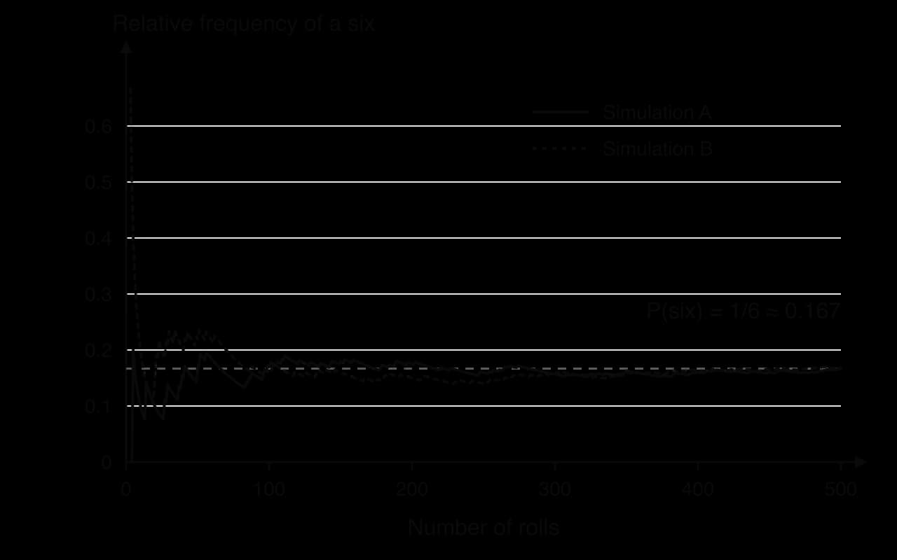
Even after 500 trials the relative frequency is only an estimate of the probability. Both runs end at a relative frequency of 0.168 (84 sixes in 500 rolls), slightly above $\frac{1}{6} = 0.1666\ldots$, and a third run would end somewhere slightly different again.

Theoretical probability and relative frequency compared

The table compares the two kinds of probability: where each comes from, how exact it is and when it can be used.

When both are available, they check each other. A large difference between a relative frequency from many trials and a theoretical probability suggests the model is wrong: the die may be biased, the selection not random, or the theory incomplete.

Case study: Mendel's peas

In experiments published in 1866, Gregor Mendel crossed pea plants that differed in one feature, such as round or wrinkled seeds. His theory said that each plant carries two copies of a heritable factor, one from each parent, and that the factor for round seeds ($R$) is dominant over the factor for wrinkled seeds ($r$). A hybrid plant $Rr$ passes on $R$ or $r$ with equal probability, so crossing two hybrids gives four equally likely combinations. This grid, known in biology as a Punnett square, is a sample space diagram.

Three of the four equally likely cells give round seeds, so the theory predicts $\mathrm{P}(\text{round}) = \frac{3}{4}$, a ratio of 3 round to 1 wrinkled. Mendel's own counts test the prediction. From 253 hybrid plants he obtained 7,324 seeds: 5,474 round and 1,850 wrinkled.

This is very close to the theoretical 0.75. The expected number of round seeds among 7,324 is $7324 \times 0.75 = 5493$, only 19 more than Mendel observed. Mendel also reported the counts for single plants, and these vary far more, as expected when each plant gives only a few dozen seeds.

Source: G. Mendel, "Experiments in Plant Hybridization" (1866), Experiment 1, English translation, MendelWeb.

On single plants the relative frequency ranges from 0.655 (plant 4, with 29 seeds) to 0.824 (plant 9, with 34 seeds), and Mendel noted even more extreme plants elsewhere, one with 43 round and 2 wrinkled seeds and another with 14 round and 15 wrinkled. Pooling the ten plants gives 336 round out of 437, a relative frequency of 0.769, and pooling all 253 plants gives 0.747. The pattern matches the simulated die. As more trials are combined, the relative frequency comes closer to the theoretical probability. The close agreement between the pooled counts and the predicted 3 : 1 ratio was strong evidence for Mendel's model of inheritance, which later became one of the foundations of genetics.

Simulation

A simulation imitates a random process with random numbers instead of carrying it out for real. It is useful when the real experiment is slow, expensive or dangerous, and when the theoretical probability is too hard to work out.

Designing a simulation

Every simulation follows the same steps.

1. Model the situation: state the probability of each outcome of one trial.

2. Assign random numbers to outcomes in the right proportions. For a probability of 0.7, the ten digits 0 to 6 could mean "success" and 7 to 9 "failure".

3. Run the simulation: generate random numbers and record the outcome of each simulated trial.

4. Repeat many times and calculate the relative frequency of the event.

5. Interpret the relative frequency as an estimate of the probability, remembering that more repetitions give a better estimate.

Simulation with technology

A GDC or a spreadsheet produces random numbers far faster than any hand method. On a TI-84 Plus CE, MATH → PRB → randInt( gives random integers, so randInt(1,6) simulates one roll of a die. In a spreadsheet, =RANDBETWEEN(1,6) filled down 500 rows simulates 500 rolls, and =COUNTIF(A1:A500,6)/500 gives the relative frequency of a six. The two runs in the relative frequency diagram were produced in exactly this way.

Estimating π by simulation

Simulation can even estimate a number that has nothing to do with chance. Random points are chosen in a square of side 1, with each coordinate a random number between 0 and 1. A quarter circle of radius 1, centred at a corner, covers an area of $\frac{\pi}{4}$ out of the square's area of 1. Since every position in the square is equally likely, the probability that a point lands inside the quarter circle is the fraction of the area it covers.

A point $(x, y)$ is inside when $x^2 + y^2 \le 1$. The relative frequency of points inside estimates $\frac{\pi}{4}$, so four times the relative frequency estimates $\pi$.

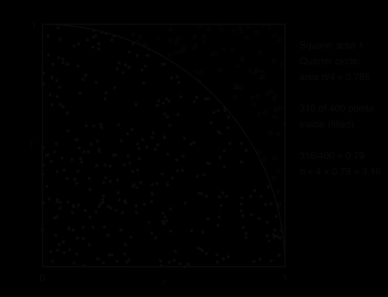
The 400 points give 3.16, already close to $\pi = 3.14159\ldots$. Continuing the same simulation to 10,000 points gave 7,874 inside, so $\pi \approx 4 \times 0.7874 = 3.1496$. The estimate improves slowly: each extra correct decimal place needs roughly a hundred times as many points. This kind of calculation, estimating a quantity from many random trials, is called a Monte Carlo method, and it is used to price financial products, model the spread of disease and design nuclear reactors.

Complementary events

Every event has an opposite. If $A$ is "the die shows a six", then "the die does not show a six" happens exactly when $A$ does not. The two events share no outcomes and together cover the whole sample space.

The Venn diagram of an event and its complement shows the sample space as a rectangle and the event as a circle inside it; $A'$ is everything in the rectangle outside the circle. Venn diagrams with two or more events are developed in subtopic 4.6.

The complement rule

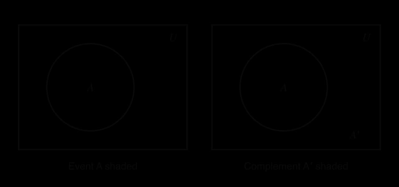
Every outcome lies either in $A$ or in $A'$, and never in both. With equally likely outcomes this means $n(A) + n(A') = n(U)$, and dividing by $n(U)$ gives the complement rule. The rule holds for every probability, including those estimated from data, because one of $A$ and $A'$ is certain to happen.

The rule saves time whenever the complement is simpler than the event itself. The clearest case is "at least one": the complement of "at least one six in two rolls" is "no sixes", which is one easy calculation instead of several.

Wording the complement correctly

The complement of an event described with an inequality or with "at least" or "at most" needs care. The complement must contain exactly the outcomes the event leaves out, no more and no fewer.

Using the complement rule backwards finds a missing probability. If the probabilities of all but one outcome are known, the last one is 1 minus their sum, because the probabilities of all the outcomes in the sample space add up to 1. Subtopic 4.7, Discrete random variables, uses this to complete probability distribution tables.

Expected number of occurrences

A probability describes one trial. Planning usually needs to know what to expect over many trials: how many students will be absent, how many components will fail, how many policyholders will claim. The expected number answers this directly.

The formula reverses the relative frequency idea. Over many trials, the event occurs in a proportion $\mathrm{P}(A)$ of them, so in $n$ trials it is expected to occur about $n \times \mathrm{P}(A)$ times. If the probability that a student is absent on a given day is 0.1, then in a class of 128 students the expected number absent is $128 \times 0.1 = 12.8$.

The answer 12.8 is not a whole number. No single day will have 12.8 absent students, but over many days the average number absent will be close to 12.8. An expected number is a long-run average, so it does not need to be a whole number and should not be rounded unless the question asks for it. It is also not a guarantee: on a particular day 9 or 16 students might be absent.

Expected numbers in life insurance

Insurers and pension funds rely on expected numbers. A national life table lists, for each age, the probability that a person of that age dies within the next year. Multiplied by the number of people insured at that age, it gives the expected number of deaths, and so the expected cost of claims. The table gives a few values from the life tables for the United Kingdom.

Source: Office for National Statistics, National life tables: United Kingdom, period 2022–2024 (published 2025).

The survivor columns start from 100,000 births and apply each year's probability of death in turn, so dividing by 100,000 turns them into probabilities of survival. They give, for example, $\mathrm{P}(\text{a newborn boy reaches 65}) \approx \frac{86\,195}{100\,000} \approx 0.862$, assuming the death rates of 2022–2024 continue. That assumption is the main limitation of a period life table: death rates usually fall over time, so the probabilities for people born today are likely to be underestimates of survival.

Exam focus

Basic probability is examined mostly in short Paper 1 questions of 3–6 marks and in the opening parts of Paper 2 questions, often before a binomial, normal or chi-squared part. Typical shapes are: probabilities read from a two-way table of survey data; a sample space diagram for two dice or a die and a spinner, followed by probabilities of totals or products; finding a missing probability because all the probabilities add up to 1; and an expected number of occurrences, $n \times \mathrm{P}(A)$, in context. The command terms are mostly write down, find, calculate, complete and explain. Single probabilities from a table usually earn one mark for the numerator and one for the denominator, so the fraction should be written before converting it to a decimal. Answers may be given as fractions, decimals or percentages, exact or to 3 significant figures.

Questions often lead from probability into a later topic: an expected number with a binomial probability (subtopic 4.8), or the expected frequencies of a chi-squared test (subtopic 4.11). In each case the expected number equals the number of trials multiplied by the probability.

Comments on relative frequency need a comparison with numbers and a reason. "The spinner is biased" with no comparison earns nothing; "0.172 is higher than the theoretical 0.125, so the spinner may favour high numbers, though 180 games is a small number of trials" earns the reasoning mark and the conclusion.

Practice questions

1. A letter is chosen at random from the word PROBABILITY. Find the probability that it is (a) a B, (b) one of the vowels A, I, O, (c) not an I. [4]

2. Two fair six-sided dice are rolled and the scores are multiplied. Find the probability that the product is (a) 12, (b) odd. [4]

3. A drawing pin is dropped 250 times and lands point up 165 times. Calculate the relative frequency of landing point up, and estimate the number of times it would land point up in 1,000 drops. [3]

4. The probability that a commuter's bus is late on any working day is 0.06. Calculate the expected number of late buses in 220 working days. [2]

5. A gym records its 240 members by membership type and age group.

A member is chosen at random. Find the probability that the member (a) has Premium membership, (b) has Standard membership and is over 50, (c) is not under 30. (d) The gym expects 900 new members with the same proportions. Find the expected number of new Premium members. [7]

6. For an event $A$, $\mathrm{P}(A') = 3\,\mathrm{P}(A)$. Find $\mathrm{P}(A)$. [2]

7. In a hypothetical country, the probability that a man aged 85 dies within a year is 0.084. (a) Write down the probability that he survives the year. (b) Calculate the expected number of deaths within a year in a group of 3,200 men aged 85. [3]

8. A student spins a spinner with five equal sectors 10 times and gets "red" 4 times, although only one sector is red. Explain why this does not show that the spinner is biased, and state what the student should do. [2]

9. Two fair coins are tossed. A student says that there are three outcomes (two heads, two tails, one of each), so $\mathrm{P}(\text{one head and one tail}) = \frac{1}{3}$. Explain the error and find the correct probability. [3]

10. In a simulation, 2,000 random points are chosen in a square of side 1 and 1,566 lie inside the quarter circle $x^2 + y^2 \le 1$. Find the estimate of $\pi$ given by the simulation and explain how the estimate could be improved. [3]

Summary

• A trial is one performance of a random experiment; each trial has one outcome; the sample space $U$ is the set of all outcomes and an event is a set of outcomes.

• Sample spaces can be shown as lists, sample space diagrams (grids for two stages) or tables of counts; with random selection from a table, $n(U)$ is the grand total.

• For equally likely outcomes, $\mathrm{P}(A) = \frac{n(A)}{n(U)}$; the formula fails when the outcomes counted are not equally likely.

• Every probability lies between 0 (impossible) and 1 (certain).

• Relative frequency = frequency ÷ number of trials; it estimates the probability and gets closer to it as the number of trials grows.

• A simulation uses random numbers to imitate a process and estimates probabilities from relative frequencies.

• Complement rule: $\mathrm{P}(A') = 1 - \mathrm{P}(A)$; it is the quickest route to "at least one".

• Expected number of occurrences in $n$ trials is $n \times \mathrm{P}(A)$, a long-run average that need not be a whole number.

Self-check

• To do:

  I can identify the trial, outcomes, sample space and an event in a described experiment.

• To do:

  I can list a sample space systematically, without missing or repeating outcomes.

• To do:

  I can draw a sample space diagram for two dice, or a die and a spinner, using sums, products or another rule.

• To do:

  I can find a probability from a two-way table of counts, using the grand total for a random choice.

• To do:

  I can use $\mathrm{P}(A) = \frac{n(A)}{n(U)}$ and explain why it needs equally likely outcomes.

• To do:

  I can explain why the totals on two dice are not equally likely.

• To do:

  I can calculate a relative frequency and use it to estimate a probability.

• To do:

  I can explain why relative frequency approaches the theoretical probability as trials increase, and why small samples vary.

• To do:

  I can compare a relative frequency with a theoretical probability and comment on possible bias.

• To do:

  I can design and carry out a simple simulation with random digits or technology.

• To do:

  I can find the probability of a complementary event, including "at least one".

• To do:

  I can write the complement of an event with "at least", "at most", "more than" or "fewer than" correctly.

• To do:

  I can find a missing probability from the fact that all probabilities add up to 1.

• To do:

  I can calculate an expected number of occurrences and explain why it need not be a whole number.

• To do:

  I can use a life table to find a probability and an expected number of deaths, and state the assumptions behind it.

[2]2 marks