4.4 Correlation and regression

Introduction

Many questions in science, economics and everyday life are about two quantities at once: whether taller people have longer arms, whether rainfall drops further from the sea, whether winning times in a race keep falling. Data of this kind are pairs of measurements, and the tools of correlation and regression describe how the two measurements move together. A scatter diagram shows the pattern, a single number, Pearson's $r$, measures how close the pattern is to a straight line, and a regression line turns the pattern into an equation that can predict one quantity from the other.

These tools are among the most widely used in applied mathematics, from medicine to economics, and they are also easy to misuse. A strong correlation does not show that one variable causes the other, a straight line does not fit a curved pattern, and a prediction far outside the data can be absurd. Using correlation and regression well therefore means knowing the conditions under which their results can be trusted, as well as the methods themselves.

Bivariate data and scatter diagrams

Most data sets met so far record one quantity for each individual: a height, a time, a score. When two quantities are measured on each individual, the data come in pairs, and the interest shifts from each variable on its own to the relationship between them.

One variable is usually chosen to explain or predict the other. The variable used to predict is the independent variable, written $x$ and plotted on the horizontal axis. The variable being predicted is the dependent variable, written $y$ and plotted on the vertical axis. In a study of how a car's fuel use depends on its speed, speed is independent and fuel use is dependent. The choice is part of the modelling: it depends on which quantity is known and which one is wanted.

The points are never joined. Each point is a separate individual, and the order of the individuals has no meaning, so a line from one point to the next would suggest a connection that does not exist. Scales should cover the data without wasting space, and they need not start at zero: if every height lies between 150 cm and 190 cm, an axis from 0 to 190 squeezes all the points into a thin strip.

Drawing a scatter diagram by hand

A scatter diagram drawn on paper follows the same rules as any accurate graph.

1. Choose which variable is $x$ and which is $y$, and label each axis with the variable's name and units.

2. Choose a scale for each axis that covers the smallest and largest values, with equal steps. Where an axis does not start at zero, it is common to show a small zig-zag break near the origin.

3. Plot each pair as a small cross or dot, reading both coordinates carefully.

4. Count the plotted points to check that none has been missed.

Describing correlation

A scatter diagram is described by the pattern its points make. Three features matter: whether the points follow a straight line or a curve, which way the trend goes, and how tightly the points cluster around it.

Unless stated otherwise, the word correlation refers to a linear pattern, in which the points cluster around a straight line.

Direction

The direction of the trend is the first thing to describe.

The opposite trend, with one variable tending to fall as the other rises, is negative correlation.

If the points show no upward or downward trend, there is no correlation (or zero correlation): knowing $x$ gives no information about whether $y$ is likely to be large or small.

Strength

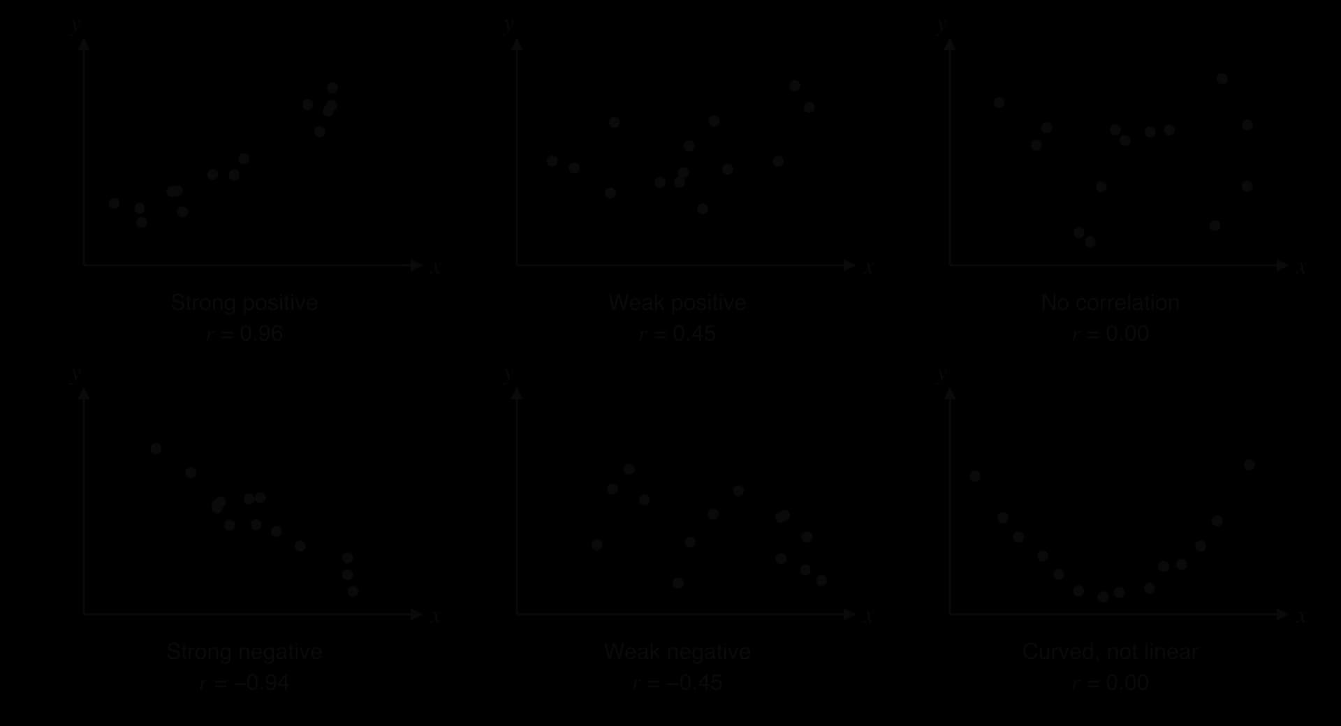
Strength describes how closely the points follow the line. When the points lie close to a straight line, the correlation is strong. When they are spread widely around it, with only a general tendency to rise or fall, it is weak. The scatter diagrams of six data sets show the main patterns side by side.

The last diagram in the set has a clear pattern: the points fall and then rise along a smooth U-shaped curve. The relationship is strong, but it is not linear, and a measure of linear correlation gives a value of about 0. Describing the shape (linear or curved) comes before describing the strength.

Pearson's product-moment correlation coefficient

Words such as "strong" and "weak" are imprecise. A single number that measures linear correlation makes descriptions comparable between data sets.

The sign of $r$ gives the direction and its size $|r|$ gives the strength. A value of $-0.95$ shows a stronger linear relationship than $+0.80$, because $0.95$ is closer to 1; the minus sign only shows that the trend is downward.

Where the formula comes from

The idea behind $r$ can be seen by dividing a scatter diagram into four regions with a vertical line at the mean $\bar{x}$ and a horizontal line at the mean $\bar{y}$. For each point, the deviations $x - \bar{x}$ and $y - \bar{y}$ measure how far it lies to the right of $\bar{x}$ and above $\bar{y}$.

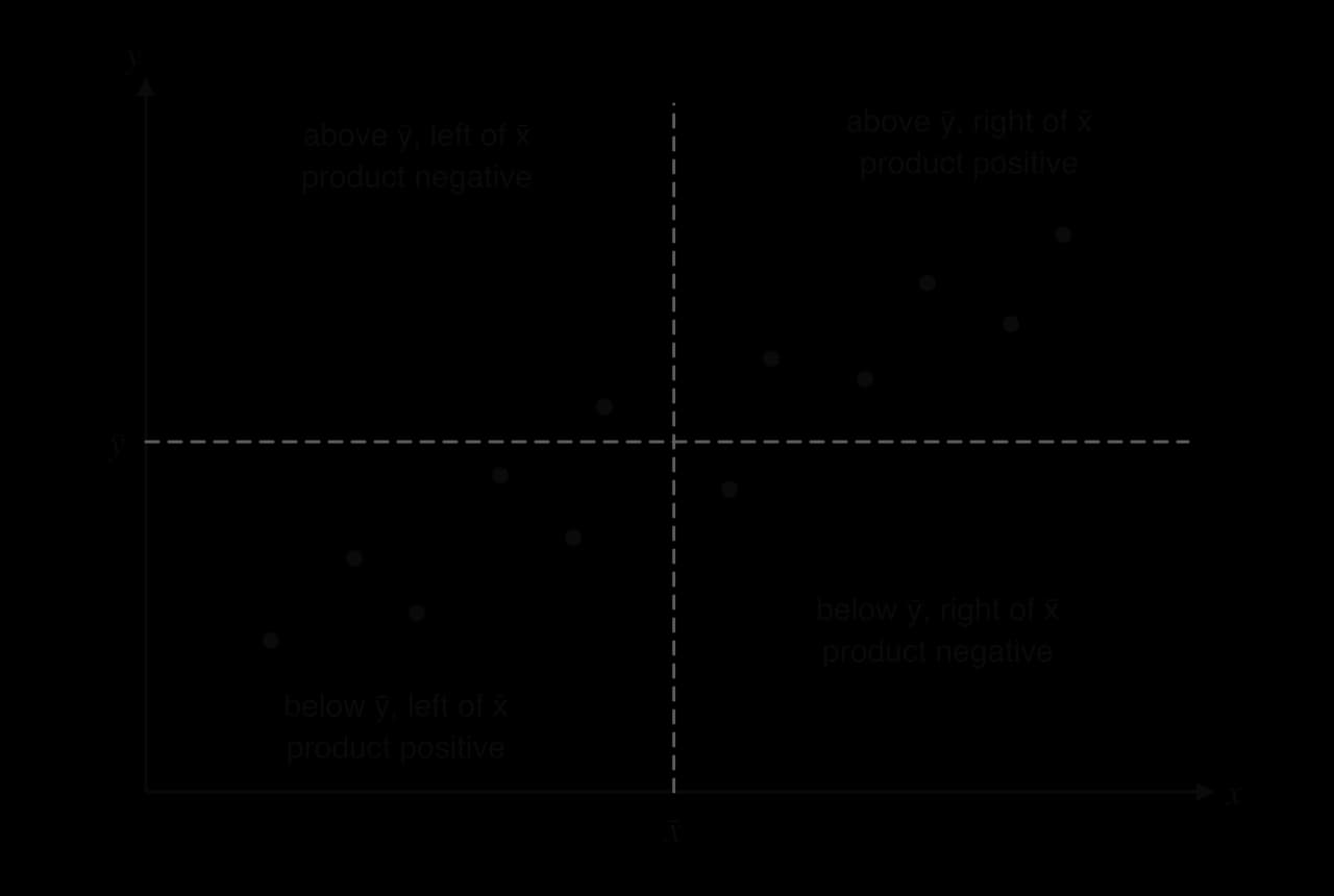
For a point in the top-right region both deviations are positive, so their product $(x - \bar{x})(y - \bar{y})$ is positive. Both deviations are negative in the bottom-left region, and the product is again positive. The other two regions give deviations with opposite signs, and so a negative product. Data with positive correlation put most points in the "positive" regions, so the sum of the products is large and positive; negative correlation gives a large negative sum; no correlation scatters the points over all four regions and the positive and negative products roughly cancel.

The sum of products depends on the units (centimetres give larger values than metres) and on how many points there are. Dividing by a quantity built from the spreads of $x$ and $y$ removes both effects and keeps the result between $-1$ and $1$. Writing $S_{xx}$, $S_{yy}$ and $S_{xy}$ for the sums of squared deviations and of products:

The GDC calculates $r$ directly, so the formula is not needed in practice. Working through it once on a small data set shows what the number measures.

Finding r with a GDC

The GDC finds $r$ as part of its linear regression function.

1. Enter the $x$-values in one list and the matching $y$-values in a second list, in the same order. Each pair must stay together.

2. Run the linear regression function $y = ax + b$ on the two lists. On a TI-84 Plus CE: STAT → CALC → LinReg(ax+b), with statistics diagnostics switched on in the MODE screen so that $r$ is shown. On a Casio fx-CG50: MENU → Statistics, then CALC → REG → X → ax+b. On a TI-Nspire: in a Lists & Spreadsheet page, Menu → Statistics → Stat Calculations → Linear Regression (mx+b).

3. Read $r$ from the output screen. The same screen gives the gradient, the intercept and $r^2$.

The screen also shows $r^2$, which is a different quantity (HL students meet it as the coefficient of determination in subtopic 4.13). The correlation coefficient is $r$, with its sign.

Interpreting the value of r

The StatQuest video shows how $r$ changes as the points spread out from a line. To turn a value into words, many textbooks use a scale like the one in the table. The boundaries are a convention, and when a different scale is supplied with a problem, that scale is the one to use.

A full description gives both features and the context: "$r = -0.981$, so there is a strong negative linear correlation between distance travelled and range: scooters that have travelled further tend to have a shorter range." The context sentence states what the number means for the scooters themselves.

Changing the units of either variable does not change $r$. Measuring heights in metres instead of centimetres multiplies every deviation by the same factor, and that factor cancels in the formula. Swapping $x$ and $y$ does not change $r$ either, since the formula is symmetric in the two variables.

Critical values of r

A value of $r$ comes from the data that happened to be collected, usually a sample. With very few points, a fairly large $r$ can appear by chance even when the two variables are unrelated: any two points with different $x$- and $y$-values lie exactly on a line, so they always give $r = \pm 1$, and three or four points can easily line up by chance. A larger sample makes a large $r$ harder to produce by chance.

A critical value of $r$ is the threshold for a given number of pairs $n$ and a given significance level. If $|r|$ is greater than the critical value, the linear correlation is unlikely to be due to chance alone and is called significant. Critical values come from tables; the table shows how the critical value falls as $n$ grows (at the 5% level, for a correlation in either direction).

With five students, $r = 0.85$ would not be enough to rule out chance, because it is less than 0.878. With fifteen students, $r = 0.55$ would be enough. The comparison uses $|r|$, so a negative $r$ is compared through its size: for the eight scooters, $|-0.981| = 0.981 > 0.707$, and the negative correlation is significant.

What r cannot show

Pearson's $r$ measures linear correlation only. A strong curved relationship can have $r$ close to 0, as the U-shaped data set in the scatter diagrams of six patterns shows, and a moderately curved one can still give a large $r$ even though a straight line is the wrong model. The value of $r$ should never be interpreted without first looking at the scatter diagram.

A single unusual point can also change $r$ dramatically. An outlier far from the trend pulls $r$ towards 0; an isolated point far from the others in the $x$-direction can create a large $r$ on its own. Checking the scatter diagram for points like these, and asking whether they are recording errors, is part of every correlation analysis. Anscombe's quartet, four data sets that share the same $r$ and the same regression line, shows all of these effects.

Correlation and causation

A strong correlation shows that two variables tend to change together, but it gives no information about why they do. The change in one variable may cause the change in the other, or there may be another explanation, and correlation alone cannot separate these possibilities.

Three situations produce a strong correlation without $x$ causing $y$.

1. The cause runs the other way. Towns with more fires tend to own more fire engines, because a town that has many fires buys more engines to deal with them; the direction of cause is from fires to engines.

2. A third variable drives both. Ice-cream sales and the number of drownings at beaches rise and fall together, because both increase in hot weather. Hot weather is a confounding variable.

3. Coincidence. Two quantities that both drift steadily over the same years are strongly correlated simply because both change with time.

The third situation is the hardest to spot. Tyler Vigen's collection of spurious correlations pairs unrelated data sets that happen to move together. In one of them, the consumption of margarine per person in the United States and the divorce rate in the US state of Maine, recorded for each year from 2000 to 2009, have $r = 0.993$. Both quantities fell over the decade for unconnected reasons, so the high value of $r$ reflects two downward trends over the same years and no link between margarine and marriage.

Source: Tyler Vigen, Spurious Correlations (tylervigen.com), using US Department of Agriculture and CDC National Vital Statistics data, accessed 2026.

Establishing causation needs more than a correlation coefficient: a controlled experiment in which one variable is changed deliberately while everything else is kept the same, or a body of evidence that rules out the other explanations. The link between smoking and lung cancer is the classic example. The British Doctors' Study recorded the smoking habits of male British doctors from 1951 and followed their causes of death until 2001; its analysis covered 34,439 men. Its 1956 report by Richard Doll and Austin Bradford Hill gave convincing statistical evidence that smoking increases the risk of lung cancer. The case for causation rested on far more than one correlation: a dose–response pattern (heavier smokers were at higher risk), a time order (smoking came before the disease), many independent studies agreeing, and a biological mechanism found by laboratory science.

Source: Doll and Hill, British Medical Journal, 1956; Doll, Peto, Boreham and Sutherland, BMJ, 2004.

The mean point and the line of best fit

When a scatter diagram shows a linear pattern, a straight line drawn through the middle of the points summarises it. Every sensible line should pass through the centre of the data.

The mean point is often labelled $M$ on a scatter diagram. It need not be one of the data points. Both coordinates come from the GDC's two-variable statistics, or from adding each list and dividing by the number of pairs.

Drawing a line of best fit by eye

1. Calculate $\bar{x}$ and $\bar{y}$, plot the mean point and label it $M$.

2. Place a ruler through $M$ and turn it until it follows the direction of the points, with the points spread evenly on the two sides of the line along its whole length.

3. Draw the line across the range of the data.

4. To estimate $y$ for a value of $x$, draw a vertical line from $x$ up to the line of best fit and a horizontal line across to the $y$-axis, and read the value.

Two people drawing by eye will produce slightly different lines, so estimates from them differ slightly too. Making every line pass through $M$ removes much of that disagreement and anchors each line at the centre of the data.

The regression line of y on x

A line drawn by eye is quick but not unique. The regression line is the one line that fits best by a precise rule, so everyone who uses the same data gets the same equation.

The least-squares idea

For each data point, the vertical distance to the line is the difference between the actual $y$-value and the value the line predicts. Some points lie above the line and some below, so the distances have both signs and would cancel if simply added. Squaring them makes every one positive and penalises large misses more than small ones. Of all possible straight lines, the regression line has the smallest total of squared vertical distances, which is why it is also called the least-squares regression line.

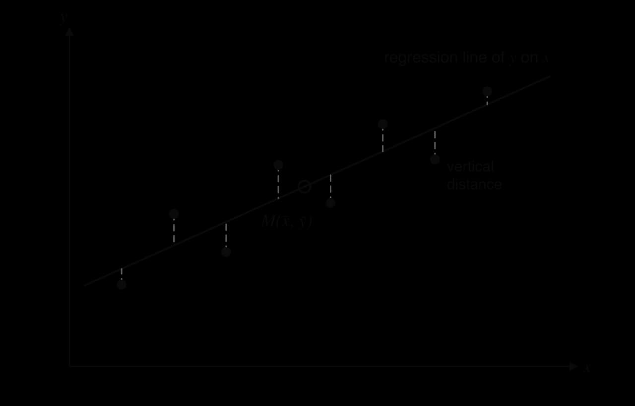
The distances in the least-squares diagram are vertical, measured in the $y$-direction, because the line is built to predict $y$. Its errors are errors in $y$, and the line makes them as small as possible.

The gradient and intercept that minimise the sum can be found with calculus. The result uses the same sums as Pearson's $r$:

Two consequences follow. Rearranging the second line gives $\bar{y} = a\bar{x} + b$, so the point $(\bar{x}, \bar{y})$ satisfies the equation: the regression line always passes through the mean point, just as a line of best fit by eye should. Also, $a$ has the same sign as $S_{xy}$, and therefore the same sign as $r$: positive correlation gives a line with positive gradient, negative correlation a line with negative gradient.

Finding the regression line with a GDC

In practice the equation always comes from the GDC.

1. Enter the $x$-values and $y$-values in two lists.

2. Run the linear regression function $y = ax + b$ (the same function that gives $r$). Some models, such as the TI-Nspire, write the line as $y = mx + b$; the gradient is then $m$.

3. Read $a$ and $b$, and write the equation using the variables of the context, with the coefficients to 3 significant figures: for the scooter data, $y = -3.64x + 51.0$.

4. Keep the full values stored in the GDC for any later calculation.

A regression line can be drawn on a scatter diagram from its equation. Two points are enough: the mean point, which lies on the line, and one other point found by substituting a value of $x$, preferably one near the edge of the data so the two points are well separated.

Interpreting the parameters a and b

In $y = ax + b$, the two numbers have meanings in the context, and stating them is part of using a regression line as a mathematical model.

The gradient $a$ is the change in $y$ for each increase of 1 unit in $x$, as in subtopic 2.1. In a regression line it is an average rate: the predicted change in $y$ per unit increase in $x$. Its units are the units of $y$ per unit of $x$. For the scooters, $a = -3.64$ means that the range falls by about 3.64 km for every additional thousand kilometres travelled.

The y-intercept $b$ is the predicted value of $y$ when $x = 0$. Whether it means anything depends on whether $x = 0$ is sensible and close to the data. For the scooters, $b = 51.0$ is the predicted range of a new scooter that has travelled 0 km, which makes sense, although $x = 0$ lies just outside the data (the smallest $x$ is 1). In many contexts $x = 0$ is impossible or far from every data point, and then $b$ only fixes the position of the line and has no meaning on its own.

Using the regression line for prediction

The main use of a regression line is to estimate a value of $y$ for a value of $x$ that was not in the data. The method is to substitute the value of $x$ into the equation, keeping the GDC's full values of $a$ and $b$.

How much an estimate can be trusted depends on two things, and both must hold.

1. The correlation must be strong. If the points are widely scattered about the line, the actual value of $y$ could be far from the line's prediction. A prediction from a weak correlation is unreliable however carefully it is calculated.

2. The value of $x$ must lie within the range of the data. Estimating inside the range of the data is interpolation. Estimating outside it is extrapolation, and it assumes that the linear pattern continues beyond the observed values, an assumption that often fails, particularly far into the future or near a physical limit.

When both conditions hold, the prediction is reliable (or valid). When either fails, it should be treated with caution or not used at all.

Do not use a y on x line to predict x

The regression line of $y$ on $x$ minimises the vertical distances, the errors in $y$. It is designed to predict $y$ from $x$. Rearranging it to find $x$ from a given $y$ uses the line for a job it was not built for. A line built to predict $x$ from $y$ would minimise the horizontal distances instead, and it is a different line.

For the revision data, the regression line of $y$ on $x$ is $y = 4.1x + 41.6$. The line built to predict hours from score is $x = 0.229y - 9.26$, which rearranges to about $y = 4.37x + 40.5$. Both lines pass through the mean point $(4, 58)$, but they have different gradients.

For a target score of 70, rearranging $y = 4.1x + 41.6$ gives $x = \frac{70 - 41.6}{4.1} = 6.93$ hours, while the line built for predicting hours gives $x = 0.22862\ldots \times 70 - 9.2602\ldots = 6.74$ hours. The weaker the correlation, the further apart the two lines are; only when $r = \pm 1$ do they coincide. The regression line of $y$ on $x$ is therefore used only to predict $y$, and a value of $x$ found by rearranging it is at best a rough estimate.

Extrapolation over time: Olympic 100 m winning times

Data collected over time invite extrapolation into the future, and a linear trend in time is especially easy to extend too far. The winning times of the men's 100 m Olympic final from 1972 to Paris 2024, all measured by fully automatic electronic timing, show a clear downward trend.

Source: Wikipedia, "100 metres at the Olympics" (finishing times data, Wikimedia Commons), accessed 2026. The 2020 Games were held in 2021.

Case study: Anscombe's quartet

In 1973 the statistician Francis Anscombe published four small data sets to show why data must be plotted before they are summarised. Each set has eleven points. The first three share the same $x$-values; the fourth uses $x = 8$ for every point but one.

Source: F. J. Anscombe, "Graphs in Statistical Analysis", The American Statistician, 1973 (data as tabulated in Wikipedia, "Anscombe's quartet").

Running linear regression on each set gives almost identical results. Every set has mean point $(9, 7.50)$, correlation coefficient $r = 0.816$ and regression line $y = 0.500x + 3.00$, all to 3 significant figures. On the numbers alone, the four data sets are indistinguishable: each would be described as a strong positive linear correlation with the same prediction rule.

The scatter diagrams of the four sets show four very different patterns.

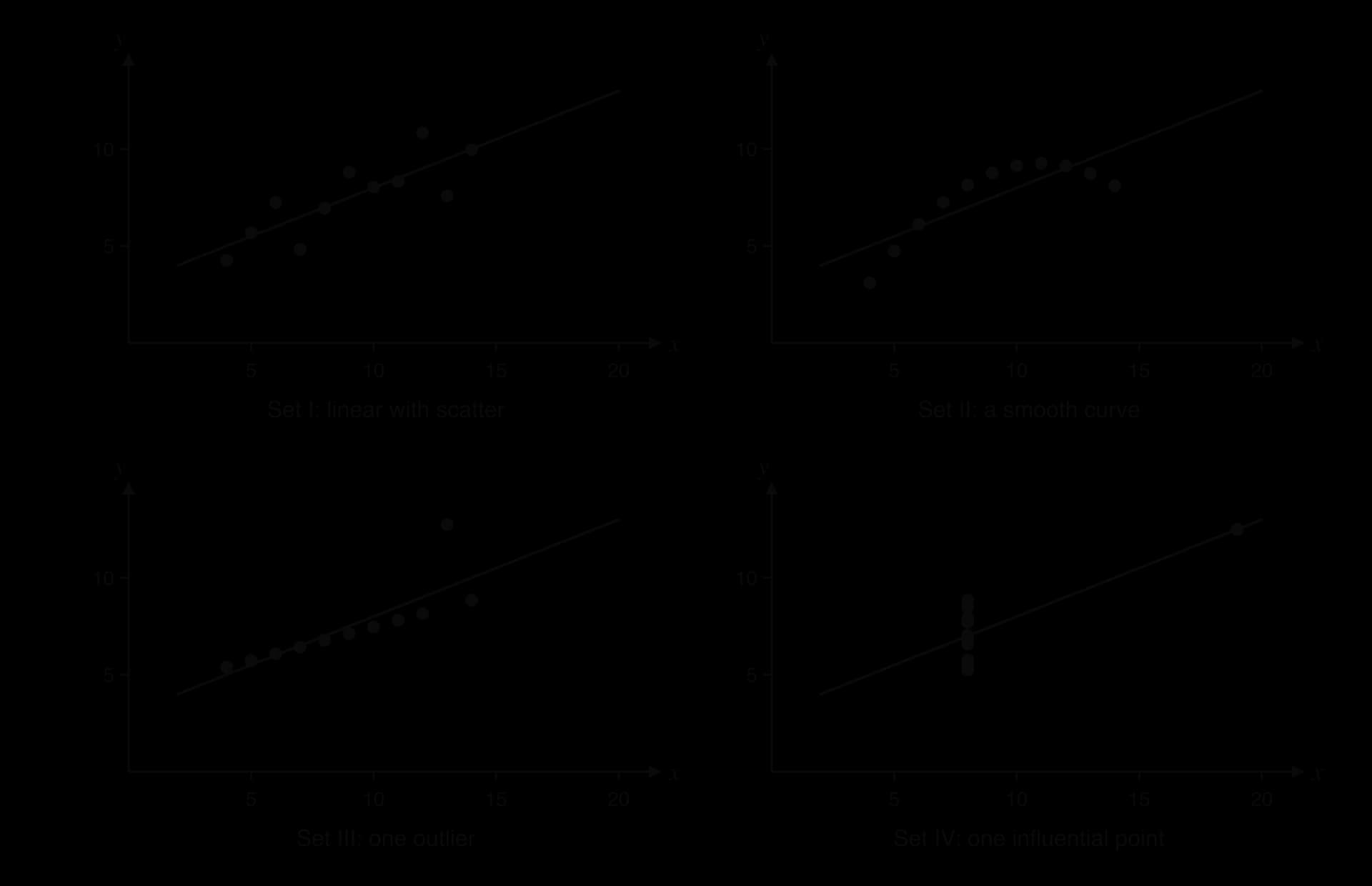
• Set I is the situation the methods are designed for: a linear trend with random scatter. Here $r = 0.816$ and the line are a fair summary.

• Set II lies on a smooth curve that rises and then falls. The relationship is almost perfect, but it is not linear, so $r$ understates it and the straight line is the wrong model. Predictions near $x = 14$ are too high and get worse beyond it.

• Set III lies exactly on a straight line except for one point, $(13, 12.74)$. Without that point, $r = 1.00$ (to 3 s.f.) and the line is $y = 0.345x + 4.01$. A single outlier has lowered $r$ and tilted the line. Before any analysis, that point should be checked: if it is a recording error it should be corrected or removed.

• Set IV has no relationship at all among the ten points at $x = 8$: they vary in $y$ with the same $x$. The single point $(19, 12.50)$ creates the entire correlation. Removing it leaves no linear trend to measure.

Anscombe's quartet leads to a rule for every correlation and regression analysis: plot the scatter diagram first. A value of $r$ and an equation summarise a pattern only after the diagram has confirmed that the pattern is linear, with no outliers or isolated points controlling the result.

Exam focus

Correlation and regression appear in almost every session, on Paper 1 as a short question of 5–8 marks and on Paper 2 as part of a longer statistics question, often combined with outliers and sampling (subtopic 4.1) or Spearman's rank correlation (subtopic 4.10). The skills are the same each time: write down or find $r$ and the regression line from a GDC, describe or interpret the correlation, estimate a value from the line, and justify or comment on whether the estimate is valid. Questions on paper may also ask you to plot and label the mean point and draw a line of best fit or the regression line.

The usual mark pattern is consistent. The value of $r$ often earns two marks, with one lost for a missing sign or wrong rounding. A regression line earns one mark for the gradient term and one for the intercept, but at most one if the answer is not written as an equation in the question's variables. A prediction earns a method mark for substituting the given value and an answer mark. A validity question needs a decision and a reason, and a decision with no reason earns nothing.

The validity question in part (g) is the most often mishandled. Two reasons can make a prediction reliable or unreliable, and markschemes often want the one that applies: strength of correlation and position within the data.

Questions also test the language of correlation itself. A description of $r$ needs both the strength and the direction, and comments must be specific.

Practice questions

1. Describe the linear correlation shown by each value of $r$: (a) $r = 0.87$; (b) $r = -0.62$; (c) $r = -0.08$. [3]

2. For the data $(2, 3)$, $(4, 7)$, $(6, 8)$, $(8, 10)$: (a) write down the mean point; (b) calculate $S_{xy}$, $S_{xx}$ and $S_{yy}$, and hence $r$, showing your working. [4]

3. A household records the daily maximum temperature, $T$ °C, and the electricity used for cooling, $E$ kWh, on eight days.

(a) Find $r$. [2] (b) Find the equation of the regression line of $E$ on $T$. [2] (c) Estimate the electricity used on a day with a maximum temperature of 28 °C. [2] (d) Comment on using the line for a day with a maximum of 45 °C. [2]

4. The cost, $C$ dollars, of a taxi journey of $d$ km is modelled by $C = 1.85d + 3.50$. Interpret the values 1.85 and 3.50 in context. [2]

5. In a sample of 10 office workers, the correlation between daily commuting time and hours of sleep is $r = -0.68$. The critical value at the 5% level for 10 pairs is 0.632. State, with a reason, whether the correlation is significant. [2]

6. A survey of 200 households finds a strong positive correlation between the number of cars a household owns and the number of overseas holidays it takes each year. Explain why this does not show that buying another car leads to more holidays. [2]

7. A biologist uses the regression line $L = 0.42m + 3.1$, where $L$ cm is the length and $m$ g the mass of a fish, to estimate the mass of a fish that is 12 cm long. Explain why this is not appropriate. [1]

8. A student records the hours of sleep, $s$, and the reaction time, $t$ milliseconds, of ten classmates.

(a) Find $r$ for all ten pairs. [2] (b) Suggest what has happened to the last pair, and find $r$ and the regression line of $t$ on $s$ without it. [4] (c) Hence estimate the reaction time of a classmate who slept 7.2 hours. [2]

Summary

• Bivariate data are pairs $(x, y)$, shown on a scatter diagram with the independent variable on the horizontal axis; the points are never joined.

• Correlation is described by its shape (linear or not), direction (positive, negative, none) and strength (strong, moderate, weak).

• Pearson's $r$, found with a GDC, measures linear correlation: $-1 \le r \le 1$, the sign gives the direction and $|r|$ the strength; it is $\frac{S_{xy}}{\sqrt{S_{xx}S_{yy}}}$.

• If $|r|$ exceeds a given critical value, the linear correlation is significant (unlikely to be chance).

• Correlation does not imply causation: reverse cause, confounding variables and coincidence all produce correlation.

• The mean point $(\bar{x}, \bar{y})$ lies on every line of best fit by eye and on the regression line.

• The regression line of $y$ on $x$, $y = ax + b$, minimises the sum of squared vertical distances; find it with a GDC and write it in the variables of the context.

• $a$ is the change in $y$ per unit increase in $x$ (with units); $b$ is the value of $y$ when $x = 0$

• A prediction is reliable only when the correlation is strong and the value of $x$ is within the data; extrapolation is unreliable, and a $y$ on $x$ line should not predict $x$.

• Always plot the data first: Anscombe's quartet shows four data sets with the same $r$ and line but different patterns.

Self-check

• To do:

  I can choose the independent and dependent variables and plot a scatter diagram with labelled axes and sensible scales.

• To do:

  I can describe a scatter diagram by its shape, direction and strength, in context.

• To do:

  I can enter paired data into my GDC and find $r$, copying $r$ (not $r^2$) with its sign.

• To do:

  I can explain what $r$ measures using the products $(x - \bar{x})(y - \bar{y})$, and calculate it by hand for a small data set.

• To do:

  I can compare $|r|$ with a given critical value and state whether the correlation is significant.

• To do:

  I can explain why $r$ is only meaningful for linear relationships and how an outlier affects it.

• To do:

  I can explain why correlation does not imply causation and suggest a confounding variable.

• To do:

  I can calculate the mean point, plot it labelled $M$, and draw a line of best fit by eye through it.

• To do:

  I can find the regression line of $y$ on $x$ with my GDC and write it as an equation in the question's variables, to 3 s.f.

• To do:

  I can draw a regression line on a scatter diagram using the mean point and one other point.

• To do:

  I can interpret the gradient and the intercept of a regression line in context with units, and say when the intercept is meaningless.

• To do:

  I can estimate $y$ from the line using the full stored values of $a$ and $b$.

• To do:

  I can justify whether a prediction is reliable using both the strength of correlation and the range of the data.

• To do:

  I can explain why a regression line of $y$ on $x$ should not be used to predict $x$.

1. (a)

   One of the temperatures has been recorded in error. Identify this value and suggest what the temperature probably was.

   [2]2 marks

   Markscheme (a)

   2.9 °C (a summer day with 168 iced drinks sold) A1

   the decimal point is misplaced; the temperature was probably 29 °C R1

   [2 marks]

2. (b)

   If the error is not noticed, the value of Pearson's product-moment correlation coefficient for all ten days is $r = 0.230$. Maya removes the day with the error.

   Find the value of $r$ for the remaining nine days.

   [2]2 marks

   Markscheme (b)

   $r = 0.956049\ldots$ ⇒ $0.956$ A2

   [2 marks]

3. (c)

   Comment on the effect of the error on the correlation coefficient.

   [1]1 mark

   Markscheme (c)

   a single incorrect value changed a strong positive correlation into what appears to be a weak one R1

   [1 mark]

4. (d)

   For the nine days, find the equation of the regression line of $n$ on $T$.

   [2]2 marks

   Markscheme (d)

   $n = 7.75T - 59.5$ ($n = 7.75232\ldots T - 59.4534\ldots$

5. (e)

   Interpret, in context, the gradient of the regression line.

   [1]1 mark

   Markscheme (e)

   for each increase of 1 °C in the maximum temperature, about 7.75 more iced drinks are sold A1

   [1 mark]

6. (f)

   Use your regression equation to estimate the number of iced drinks Maya sells on a day when the maximum temperature is 25 °C.

   [2]2 marks

   Markscheme (f)

   $7.75232\ldots \times 25 - 59.4534\ldots$ (M1)

   $134.354\ldots$ ⇒ 134 (drinks) A1

   Note: Accept $134.3$ or $134.4$

7. (g)

   Maya wants to use the equation to estimate sales on a winter day with a maximum temperature of 12 °C. Explain why this estimate may not be reliable.

   [2]2 marks

   Markscheme (g)

   12 °C is outside the range of the recorded temperatures (22 °C to 33 °C) R1

   so this is extrapolation, and the linear relationship may not continue (the model gives about 34 drinks) R1

   [2 marks]

8. (h)

   Maya says the café was closed on one day during the ten-day period, so no data were recorded. She suggests recording 0 drinks for that day. Explain why this would be inappropriate.

   [1]1 mark

   Markscheme (h)

   0 drinks was caused by the café being closed, not by the temperature, so it would distort the relationship (it is missing data, not a real observation) R1

   [1 mark]

• trend: y = −3.64x + 51.0

The points fall from left to right and lie close to a straight line. Scooters that have travelled further tend to have a shorter range, and the pattern is linear, so there is strong negative linear correlation.

Every product is positive or zero, which already suggests positive correlation.

Entering the hours in one list and the scores in another and running linear regression on a GDC gives $r = 0.968173\ldots$, the same value. There is a strong positive linear correlation between hours of revision and test score for these five students.

(b) The line is drawn through $M$ following the direction of the points, with points close to it on both sides along its whole length. One such line passes through $M(167, 168)$ and close to $(150, 152)$.

Reading up from $s = 160$ to the line and across to the vertical axis gives $h \approx 161$ cm. (M1)A1 Any answer from about 160 cm to 163 cm is reasonable, since each line by eye is slightly different.

and the intercept is

so the regression line is $y = 4.1x + 41.6$. A GDC's linear regression on the two lists gives $a = 4.1$ and $b = 41.6$, the same values.

At $x = 4$: $y = 4.1 \times 4 + 41.6 = 58$, which is $\bar{y}$. The line passes through the mean point $(4, 58)$.

A1A1 for the gradient term and the intercept, written as an equation in $t$ and $x$.

(b) The winning time falls by about 0.00843 seconds per year on average, which is about 0.034 seconds from one Games to the next. A1

(c) 2028 is $x = 56$:

The estimate is 9.65 s. (M1)A1 The correlation is strong ($r = -0.834$) and 2028 is only four years beyond the data, but it is still extrapolation, and the times since 2008 have levelled off at about 9.6–9.8 s, so the estimate is a rough guide only. R1

(d) Solving $-0.0084285\ldots x + 10.11914\ldots = 0$ gives $x = 1200.6\ldots$, so about the year 3173. A1 A time of 0 s is impossible, and the model also predicts that the Olympic winner will beat Usain Bolt's world record of 9.58 s (Berlin, 2009) by about 2036. Human speed has physical limits, so winning times must level off: the linear trend describes 1972–2024 well but cannot be extended far beyond it. R1

Award A1 for 0.949 (sign omitted) or for −0.950 (incorrect rounding).

(c) $|r| = 0.949 > 0.666$ R1

so there is significant (strong) negative linear correlation between distance from the coast and rainfall. A1

Do not award R0A1.

(d) $R = -4.80d + 1470$ $(R = -4.80215\ldots d + 1474.97\ldots)$ A1A1

Award A1 for $-4.80d$ and A1 for 1470. Award at most A1A0 if the answer is not an equation, or is written in $x$ and $y$.

(e) The mean annual rainfall decreases by about 4.80 mm for every extra kilometre from the coast. A1

(f) $R = -4.80215\ldots \times 65 + 1474.97\ldots$ (M1)

$= 1160$ mm $(1162.83\ldots)$ A1

(g) No, the line should not be used. A1

250 km is outside the range of the data (5 km to 120 km), so this would be extrapolation. R1

Do not award A1R0.

(h) The line of $R$ on $d$ is for predicting $R$ from a given $d$, not $d$ from a given $R$. R1

(i) Correlation does not imply causation: the decrease may be caused by other factors, such as height above sea level or mountains blocking moist air. R1

Total [15]

Note: Award $\mathbf{A1}$ for $7.75T$, $\mathbf{A1}$ for $-59.5$. Award at most $\mathbf{A1A0}$ if the answer is not an equation.

[2 marks]

[2 marks]

(ii) the equation of the regression line of $T$ on $x$.

[4]4 marks