Organise data in frequency tables, draw histograms and cumulative frequency graphs, read medians, quartiles and percentiles from them, and draw and compare box-and-whisker diagrams.
Each is in the Maths AI glossary, with every other term in the subject.
A diagram drawn against a scale in which a box spans the lower to the upper quartile with a line at the median, and whiskers extend from the box to the smallest and largest values that are not outliers; any outliers are marked separately with a cross.
A range of values grouped together as one class in a frequency distribution, written as an inequality such as .
The running total of the frequencies up to and including a given class, which gives the number of data values below that class's upper class boundary.
A graph of cumulative frequency (vertical axis) against the upper class boundaries (horizontal axis), with the points joined by a smooth increasing curve or by straight line segments.
The minimum, lower quartile, median, upper quartile and maximum of a data set.
Construct a frequency distribution table for discrete or continuous data, using class intervals written as inequalities without gaps.
Draw a frequency histogram with equal class intervals and interpret its shape.
Calculate cumulative frequencies and draw a cumulative frequency graph by plotting them against upper class boundaries.
Estimate the median, quartiles, percentiles, range and interquartile range from a cumulative frequency graph.
Use a cumulative frequency graph in reverse to find how many values lie above or below a given value.
Draw a box-and-whisker diagram to scale from a five-number summary, marking outliers with a cross.
Interpret box-and-whisker diagrams, including what each section does and does not show.
Compare two distributions using their medians, spreads and symmetry, in context.
Determine whether data may be normally distributed by judging the symmetry of a box-and-whisker diagram.
A list of several hundred numbers shows almost nothing at a glance. Presenting data means organising it, in a table or a diagram, so that its centre, its spread and its shape can be seen and measured. A frequency table counts how often each value or group of values occurs, a histogram turns those counts into bars, a cumulative frequency graph shows how the data build up from the smallest value to the largest, and a box-and-whisker diagram reduces a whole data set to five numbers that can be compared with another set on the same scale.
Each representation shows some features and hides others. The age structure of a country, the finishing times of thousands of runners or the life expectancies of a hundred countries can all be summarised this way, and the choice of diagram decides what a reader notices first.
27 exam-style questions on this subtopic, written in the style of the IB papers. The first has its markscheme open. Counted on
As part of a road-safety study, 40 drivers each take a computer test that measures their reaction time, in seconds. The results are summarised in the following table.
Minimum | Lower quartile | Median | Upper quartile | Maximum |
|---|---|---|---|---|
0.09 | 0.24 | 0.27 | 0.31 | 0.44 |
Write down the interquartile range.
1 mark
The entries of the mathematics: applications and interpretation formula booklet that 4.2 uses. Each opens in the explained booklet.
With a free account, Augment remembers where you stopped and what you have practiced.
The number of times a particular value, or a value within a particular group, occurs in a data set.
A table that lists each value, or each group of values, of a variable together with its frequency.
Data that have been sorted into classes, so that the table gives the number of values in each class rather than each individual value.
A diagram for grouped continuous data in which each class is shown by a bar standing on its class interval, with no gaps between bars; with equal class widths, the height of each bar is its frequency.
The difference between the upper and lower quartiles, , which measures the spread of the middle 50% of the data.
The value below which one quarter (25%) of the data lie when the data are arranged in order; it is written .
The middle value of a data set arranged in order of size, so that half of the values are less than or equal to it and half are greater than or equal to it.
The th percentile is the value below which of the data lie when the data are arranged in order.
The difference between the largest and smallest values in a data set, maximum − minimum.
A distribution that is not symmetric because its values are spread out further on one side of the centre, giving a longer tail on that side; the skew is positive when the long tail is towards larger values and negative when it is towards smaller values.
A distribution whose values are spread in the same way on both sides of its centre, so that one half of its histogram is roughly a mirror image of the other.
The value at the top end of a class interval, which is the boundary it shares with the next class.
The value below which three quarters (75%) of the data lie when the data are arranged in order; it is written .
Raw data are the values as they were recorded, in no particular order. The first step in presenting them is to count how many times each value occurs. This count is the frequency, usually written , and the full list of values with their frequencies is a frequency distribution.
A frequency distribution keeps every piece of information in the raw list while making it far easier to read. The sum of the frequencies, , always equals the number of data values , which is a useful check that nothing has been missed or counted twice.
When discrete data take only a few different values, each value gets its own row. A tally (a stroke for each value, with every fifth stroke drawn across the previous four) is a reliable way to count by hand, but only the frequencies need to appear in the final table.
Number of people in the car, | 1 | 2 | 3 | 4 | 5 |
|---|---|---|---|---|---|
Frequency, | 12 | 7 | 3 | 2 | 1 |
The table records the number of people in each of 25 cars passing a checkpoint. The frequencies add to 25, one for each car. Because the data are still ungrouped, the original values can be rebuilt exactly: there are twelve 1s, seven 2s, and so on. That means any statistic, such as the total number of people or the middle value, can still be found exactly from the table.
When data take many different values, a table with one row per value is almost as hard to read as the raw list. Continuous data such as times, masses and lengths rarely repeat at all, because every measurement is slightly different. Such data are sorted into groups called classes, and the frequency of each class is counted instead.
Each class covers an interval of values. To avoid any doubt about where a value belongs, intervals are written as inequalities, and neighbouring intervals share a boundary so that there are no gaps between them and no overlaps.
The inequality signs decide which class a value on a boundary joins. In the classes and , a time of exactly 5 belongs to the first class, because is true and is false. With the other convention, and , the same value joins the second class. Either convention is acceptable, provided every possible value belongs to exactly one class.
Way of writing the classes | Problem |
|---|---|
0–5, 5–10, 10–15 | A value of 5 could go in two classes |
0–4, 5–9, 10–14 (continuous data) | A value of 4.6 belongs to no class |
, , | None: every value has exactly one class |
The width of a class is the difference between its two boundaries, so has width 5. Choosing the classes is a compromise. Wide classes give a short table but blur the detail, while very narrow classes leave many classes with frequencies of 0 or 1 and no clear pattern. Between about 5 and 10 classes of equal width usually works well.
For classes written as inequalities, the upper class boundary is simply the larger number in the inequality. Care is needed when a class is written with whole numbers for a continuous quantity. Ages are usually recorded in completed years, so the class "30–34 years" contains everyone from their 30th birthday up to, but not including, their 35th birthday. As an inequality this is , and its upper class boundary is 35, not 34.
Grouping loses information. Once 30 phone calls are reduced to five class frequencies, the exact length of each call can no longer be recovered, so any statistic calculated from grouped data is an estimate. Subtopic 4.3 uses mid-interval values to estimate the mean of grouped data for the same reason.
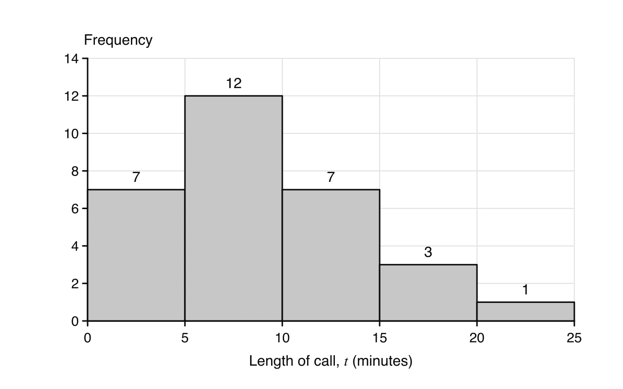
A histogram presents a grouped frequency distribution of continuous data as a set of touching bars. Each bar stands on its class interval on the horizontal axis, so the bars meet at the class boundaries with no gaps, because the variable is continuous and there are no gaps between the classes. When all the classes have the same width, the height of each bar is the frequency of its class.
A histogram differs from a bar chart in two ways. A bar chart shows categories or separate discrete values, so its bars are drawn apart and could be placed in any order. A histogram has a continuous number line along the bottom, with a scale, and each bar covers a range of that line.
The histogram of the 30 phone calls shows at once that most calls lasted between 5 and 10 minutes, that very few lasted more than 15 minutes, and that the distribution has a longer tail on the right than on the left.
Draw a horizontal axis for the variable, with a linear scale that covers every class boundary, and label it with the variable and its unit.
Draw a vertical axis labelled "Frequency", with a scale that reaches just beyond the largest frequency.
For each class, draw a rectangle from its lower boundary to its upper boundary, as high as its frequency.
Check that neighbouring bars share an edge, so there are no gaps, and that the bars are drawn with a ruler.
In a histogram the eye judges each bar by its area, not just its height. With equal class widths, area is proportional to height, so comparing heights and comparing areas give the same answer. If one class were twice as wide as the others, a bar drawn to the height of its frequency would have twice the area its frequency deserves and would look far more important than it is. That is why histograms with unequal classes use frequency density (frequency divided by class width) instead of frequency on the vertical axis, a refinement that is not needed when every class has the same width.
The same principle drove one of the most famous diagrams in the history of statistics. Florence Nightingale's polar area diagram of deaths in the British Army during the Crimean War gives each month a wedge with the same angle, and makes the area of each wedge, measured from the centre, proportional to the number of deaths. Because area grows with the square of the radius, a month with four times as many deaths has a wedge only twice as long.
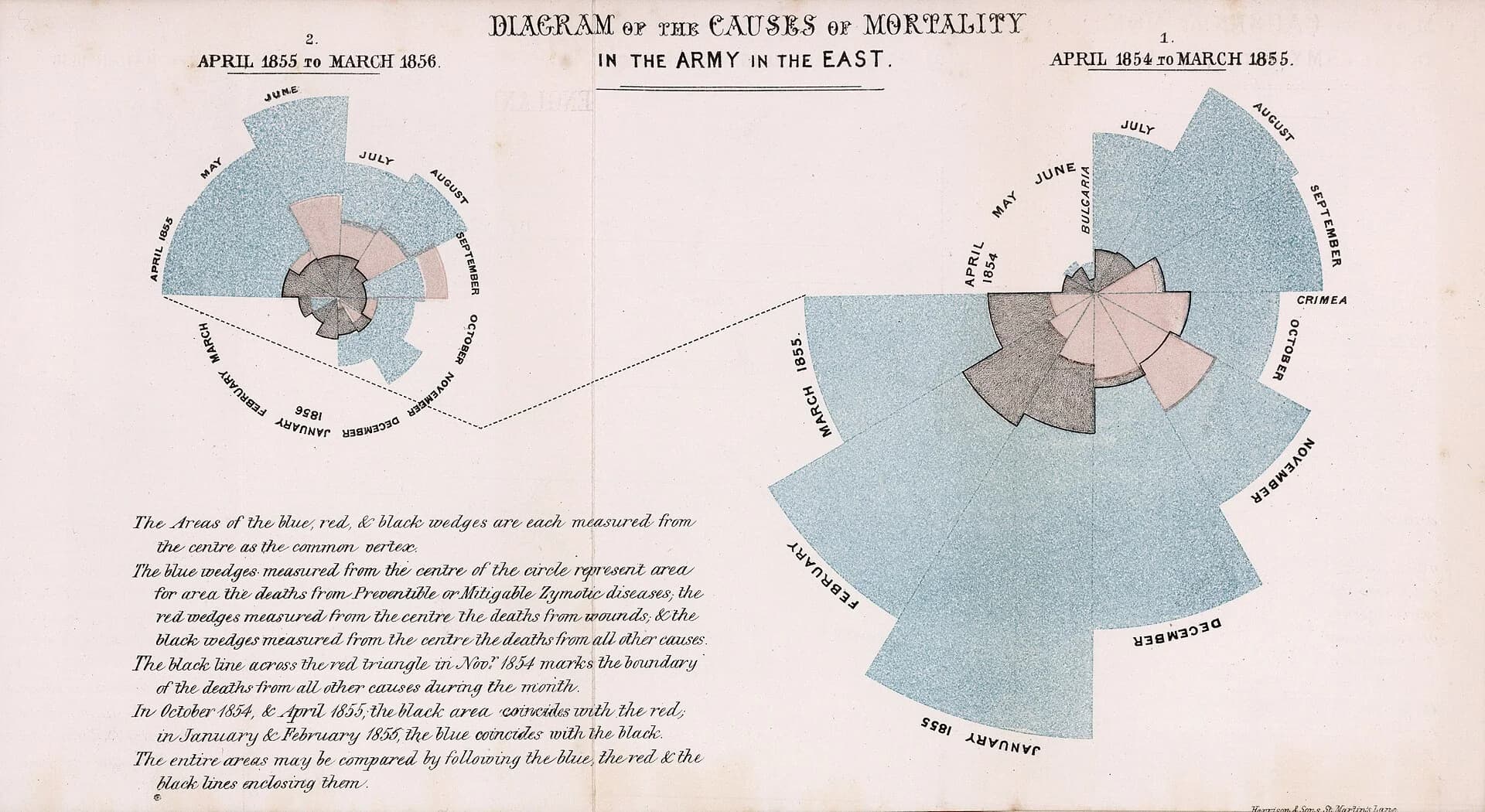
Nightingale published the diagram in 1858 in her report Notes on Matters Affecting the Health, Efficiency, and Hospital Administration of the British Army, which was sent to Queen Victoria. Its blue wedges, deaths from what she called preventable or mitigable diseases, are far larger than the red wedges for deaths from wounds. Drawing the counts as areas made that comparison visible to readers who would never have studied a table of monthly figures.
A GDC draws a histogram from a list of values, or from a list of values with a list of frequencies. Because the calculator needs a single number for each class, a convenient choice for grouped data is any value inside the class, such as the mid-interval value, entered with the class frequency.
Enter the values in one list and, for grouped data, the frequencies in a second list.
Open the statistical plot menu, switch a plot on and choose the histogram type, with the first list as the data and the second list as the frequencies.
Set the window so that the minimum value is the lowest class boundary and the bar width (on TI calculators Xscl, on Casio calculators the "width" setting) equals the class width.
Draw the graph and check the bar heights against the table.
If the bar width does not match the class width, the calculator regroups the data into different classes, and the histogram no longer matches the table.
The masses, grams, of 60 eggs from a farm (hypothetical data) are summarised in a grouped frequency table.
Mass, g | ||||||
|---|---|---|---|---|---|---|
Frequency | 3 | 9 | 17 | 18 | 10 | 3 |
Many questions about data are of the form "how many values are less than this?" or "below what value do 90% of the data lie?". A frequency table answers the first only for the boundaries of classes, and only after adding up several classes. Cumulative frequencies do this adding once, for every boundary.
To build a cumulative frequency table, start with the frequency of the first class and keep a running total, adding the frequency of each class in turn. The final cumulative frequency always equals the total number of values, .
Height, cm | ||||||
|---|---|---|---|---|---|---|
Frequency | 4 | 10 | 22 | 26 | 12 | 6 |
Cumulative frequency | 4 | 14 | 36 | 62 | 74 | 80 |
Meaning |
The table gives the heights of 80 tomato seedlings three weeks after planting (hypothetical data). The cumulative frequency 36 under means that 36 seedlings are at most 12 cm tall, because they lie in the first three classes, and all of those classes end at or before 12. That is why each cumulative frequency belongs to the upper class boundary of its class.
Plotting each cumulative frequency against its upper class boundary, and joining the points, gives a graph from which the number of values below any value can be estimated, not only below the class boundaries.
The method for drawing one:
Add a cumulative frequency row to the frequency table.
Plot the point (lowest class boundary, 0): no values lie below the start of the first class. For the seedlings this is .
Plot each point (upper class boundary, cumulative frequency): .
Join the points with a smooth curve (or with straight lines, if the question allows). The curve never goes down, because a running total can only stay the same or grow.
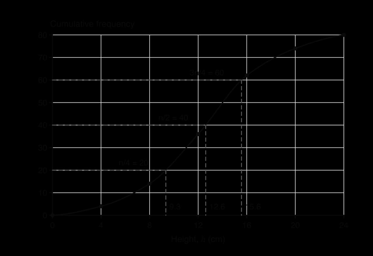
The shape of the cumulative frequency graph of the seedlings carries the same information as a histogram, in a different form. Where the curve is steep, many values are packed into a short interval, so the steepest part, between 8 and 16 cm, is where the data are most concentrated. Where it is nearly flat, near the ends, there are few values. A curve of this stretched-S shape belongs to data that cluster in the middle.
Once the data are arranged in order, values can be described by their position: the value halfway through, a quarter of the way through, or 90% of the way through. A cumulative frequency graph makes this easy, because its vertical axis is the position in the ordered data.
For a short list of values in order, the median is the th value: the 8th of 15 values, or halfway between the 10th and 11th of 20 values. For grouped data on a cumulative frequency graph, the median is read at a cumulative frequency of . The two rules differ slightly because a cumulative frequency graph treats the data as spread continuously along the axis, so exactly half of the data lie below the point at height ; with large data sets the difference is negligible, and graph readings are estimates anyway.
The median splits the data into two halves. The quartiles split each half again, so that the data fall into four parts with about a quarter of the values in each.
The median is sometimes called the second quartile, , because half of the data lie below it. The upper quartile marks the point three quarters of the way through the ordered data.
Quartiles generalise to any percentage. The 90th percentile, for example, is the value below which 90% of the data lie. The median is the 50th percentile, is the 25th percentile and is the 75th percentile.
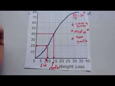
To find a value at a given position, convert the position into a cumulative frequency, then read across to the curve and down to the horizontal axis.
Statistic | Cumulative frequency to read at | Seedlings () |
|---|---|---|
Lower quartile | 20 | |
Median | 40 | |
Upper quartile | 60 | |
th percentile | 90th: |
The graph of the seedling heights gives , median and . Readings like these are estimates, accurate to about half of a small grid square, so any answer within a small range of each value is equally reasonable.
The graph also works the other way: start from a value on the horizontal axis, read up to the curve and across to the cumulative frequency, which is the number of values less than or equal to that value. The number greater than the value is then minus that reading, and the number between two values is the difference of two readings.
Finding "the value exceeded by the top 8 items" is also a matter of position. The top 8 of 80 lie above a cumulative frequency of , so the value is read at 72, exactly as for the 90th percentile.
The median and the quartiles locate the data. Two further measures describe how spread out the data are.
The range is simple, but it depends only on the two most extreme values, so a single unusual value can make it very large. The interquartile range avoids this by measuring the spread of the middle half of the data, ignoring the lowest quarter and the highest quarter.
A cumulative frequency graph gives a good estimate of the IQR, but only a rough idea of the range. The graph starts at the lowest class boundary and finishes at the highest, while the actual smallest and largest values lie somewhere inside the first and last classes. For the seedlings, the range is less than , but its exact value is unknown unless the minimum and maximum are given separately.
The IQR is the measure used most with the median, and it underlies the outlier test of subtopic 4.1: a value more than below or above is classed as an outlier.
 YouTube
The median, the two quartiles, the minimum and the maximum together describe where a data set sits, how spread out it is, and whether it is balanced. These five values are called the five-number summary.
A box-and-whisker diagram (also called a box plot) draws the five-number summary to scale against a number line. The box runs from to with a vertical line at the median, and a whisker extends from each end of the box towards the extreme values.
Each of the four sections of the diagram, the left whisker, the two parts of the box and the right whisker, contains about a quarter of the data. The box itself holds the middle 50%, so its length is the IQR, and the distance from the end of one whisker to the end of the other (including any outliers) is the range.
A whisker drawn all the way to an outlier would make the data look far more spread out than they are. So, when a data set contains outliers, each whisker stops at the most extreme value that is not an outlier, and each outlier is drawn as a cross at its own position. The test for an outlier uses the fences of subtopic 4.1.
Any value below the lower fence or above the upper fence is an outlier. The fences themselves are not drawn on the final diagram; they only decide where the whiskers end.
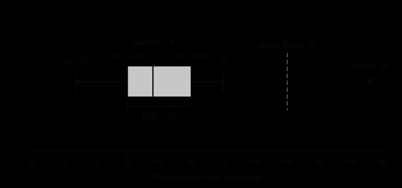
For a short list of values, the five-number summary can be found by hand, and the method shows what a GDC does.
Put the values in order and find the median: the th value.
Split the data into a lower half and an upper half. When is odd, leave the median out of both halves.
is the median of the lower half and is the median of the upper half.
Check for outliers using the fences, then draw the diagram.
A box-and-whisker diagram is a scale drawing, not a sketch. The steps:
Draw a horizontal axis with a linear scale that covers the minimum and maximum, and label it with the variable and its unit.
Draw vertical lines at , the median and , all the same height, and join the ends of the outer two to make the box.
Draw the whiskers as horizontal lines from the middle of each end of the box to the smallest and largest values that are not outliers, with short vertical lines at their ends.
Mark any outlier with a cross at its position, level with the whiskers.
The median line goes only across the box. A single horizontal line drawn right through the box, from one whisker to the other, is a common error.
A GDC finds the five-number summary of raw data with its one-variable statistics function and draws the diagram as a statistical plot.
Enter the data in a list (with a frequency list if the data are in a frequency table).
Run one-variable statistics (on a TI-84 Plus CE: STAT → CALC → 1-Var Stats; on a Casio fx-CG50: MENU → Statistics → CALC → 1-VAR). Scroll to read the minimum, , the median, and the maximum.
For the diagram, switch on a statistical plot and choose the box plot type. Most calculators offer two: the modified box plot marks outliers as separate points and stops the whiskers at the most extreme non-outliers, while the plain version runs the whiskers to the minimum and maximum.
Calculators, spreadsheets and textbooks do not all use the same rule for the quartiles of raw data, so they can give slightly different values of and for the same small data set; subtopic 4.3 returns to this. For large data sets the differences are negligible.
A box-and-whisker diagram also hides a lot. Individual values cannot be read from it (except the five in the summary and any outliers), so it cannot show gaps, clusters or two separate peaks, and it gives no information about the number of values. A histogram or a list of the data is needed for those.
 YouTube
The overall pattern of a histogram or a box-and-whisker diagram is called the shape of the distribution. Shape matters because it affects which summary statistics describe the data fairly, and because many statistical models, such as the normal distribution of subtopic 4.9, assume a particular shape.
In a symmetric distribution the median lies in the middle of the box of the box-and-whisker diagram, and the two whiskers are about the same length. When the values spread out further on one side than the other, the distribution is skewed, and it is named after the side with the long tail.
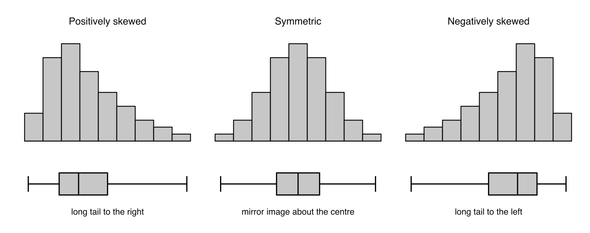
Feature | Positive skew | Symmetric | Negative skew |
|---|---|---|---|
Long tail of the histogram | Right (large values) | Neither side | Left (small values) |
Position of the median in the box | Nearer | In the middle | Nearer |
Longer whisker | Right | Neither | Left |
Examples | Incomes, house prices, phone call lengths | Heights of adults of one sex, measurement errors | Scores on an easy test, ages at death in a rich country |
The histogram of phone call lengths is positively skewed: most calls are short, a few are long, and calls cannot be shorter than 0 minutes. Data with a natural lower limit and no upper limit are often skewed this way.
The normal distribution, taught in subtopic 4.9, is symmetric and bell-shaped, with most values near the centre and fewer towards each end. A box-and-whisker diagram gives a quick check of whether data may be normally distributed:
the median is close to the middle of the box, so ;
the two whiskers are of similar length;
the whiskers are longer than each half of the box, since normal data thin out gradually towards the ends.
A strongly skewed box-and-whisker diagram rules out a normal model. A symmetric one does not prove that the data are normal, because many symmetric distributions are not bell-shaped, so the conclusion is always that the data "may be" or "could be" normally distributed.
Box-and-whisker diagrams drawn one above the other on the same scale are the standard way to compare two or more data sets. A good comparison covers three things and always refers to the context:
Centre: compare the medians, saying which group has the higher typical value.
Spread: compare the IQRs (or ranges), saying which group is more consistent; a smaller IQR means the middle half of the data are closer together.
Shape: comment on symmetry or skew, and on any outliers.
The comparison must name the statistic used. A box-and-whisker diagram shows medians, not means, so a statement such as "group A has the higher mean" cannot be justified from it.
The five-number summaries of life expectancy at birth in 2023 for the economies of two World Bank regions are given in the table; each economy (a country or territory) is one data value.
Region | Number of economies | Minimum | Median | Maximum | ||
|---|---|---|---|---|---|---|
Sub-Saharan Africa | 48 | 54.5 | 61.85 | 64.1 | 67.4 | 76.1 |
Europe & Central Asia | 58 | 70.1 | 75.8 | 79.7 | 82.5 | 86.4 |
Source: World Bank, World Development Indicators (SP.DYN.LE00.IN), 2023 values, accessed 2026; quartiles calculated from the values to 1 decimal place.
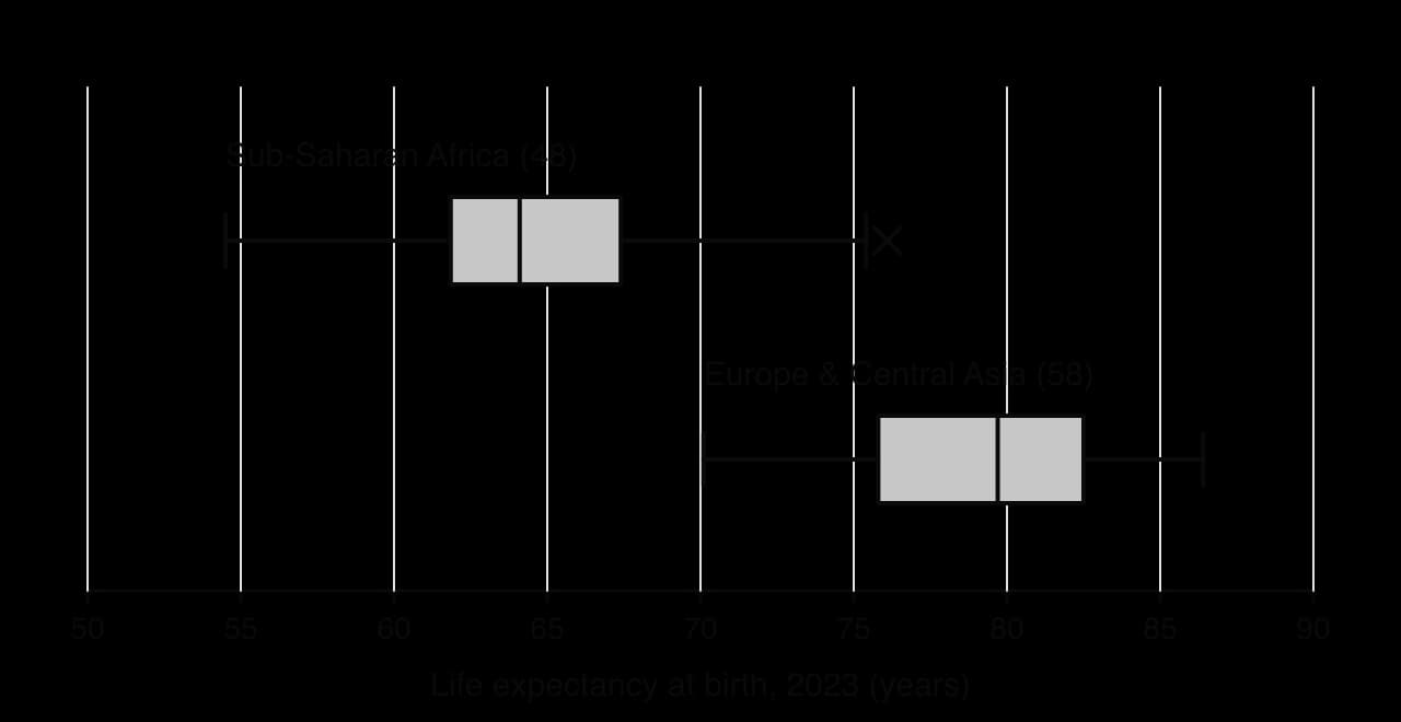
The two box-and-whisker diagrams of life expectancy make the difference between the regions visible in a way that a list of 106 numbers cannot. They also show its limits: each value is one economy, whether it has fewer than 40,000 people (Monaco, San Marino) or more than 200 million (Nigeria), so the diagrams compare countries and territories, not people.
Population age distributions show grouped continuous data on a national scale. The World Bank publishes the population of every country in 5-year age groups. In 2023 Japan had one of the oldest populations in the world and Niger one of the youngest.
Age group (years) | Japan (millions) | Niger (millions) |
|---|---|---|
4.15 | 4.67 | |
4.95 | 4.08 | |
5.41 | 3.54 | |
5.68 | 2.95 | |
6.08 | 2.38 | |
6.09 | 1.86 | |
6.16 | 1.46 | |
6.89 | 1.19 | |
7.67 | 0.99 | |
9.28 | 0.79 | |
9.66 | 0.64 | |
8.16 | 0.53 | |
7.54 | 0.41 | |
7.39 | 0.30 | |
8.76 | 0.20 | |
7.81 | 0.11 | |
12.85 | 0.06 | |
Total | 124.52 | 26.16 |
Source: World Bank, World Development Indicators (population by 5-year age group, male plus female, SP.POP.0004.MA … SP.POP.80UP.FE), 2023 values, accessed 2026. Figures rounded to the nearest 0.01 million, so columns may not add exactly to the totals.
The age groups published as "0–4", "5–9" and so on contain everyone up to the next birthday, so they are written as the classes , , …, each of width 5 years, with upper class boundaries 5, 10, 15, and so on. The last class, 80 and over, is open: it has no upper boundary. A histogram with equal class widths cannot include it, so the histograms of the two populations stop at age 80.
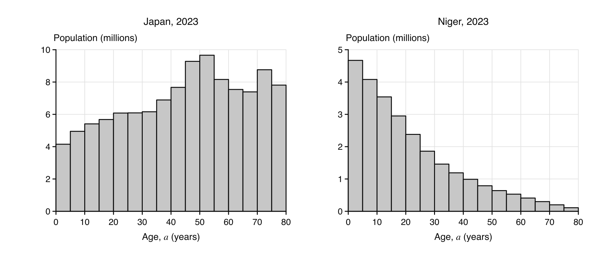
The shapes are opposite. In Niger each age group is smaller than the one before it, so the distribution of ages is strongly positively skewed, the pattern of a population with high birth rates. In Japan the youngest groups are the smallest and the bars grow towards the 45–55 age groups, people born between the late 1960s and the late 1970s, with a second peak at 70–75 and, beyond the histogram, a very large open class of 12.85 million people aged 80 and over. Most of Japan's population is therefore in the middle and older classes, with the smaller young classes on the left, a mild negative skew.
Adding the frequencies for Japan gives the cumulative frequency at each upper class boundary: 4.15 million at 5, 9.09 million at 10, and so on up to 111.67 million at 80. The remaining 12.85 million people are aged 80 or over, so the cumulative frequency graph can be drawn up to age 80 but not beyond, because the last class has no upper boundary.
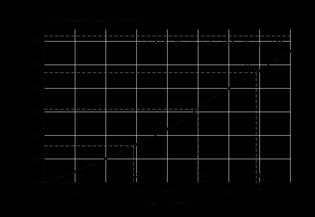
With million, the median is read at million and the quartiles at million and million.
Half of Japan's population was aged about 50 or over in 2023. The same method for Niger, whose total is 26.16 million, gives a median age of about 16 years, with quartiles of about 7 and 30 years (IQR about 23 years): half of the population of Niger was under about 16.
The open class limits what the graph can give. The 90th percentile of Japan's ages lies at a cumulative frequency of million, which is beyond 111.67 million, the cumulative frequency at age 80. So the 90th percentile is somewhere above 80, and the graph cannot say where. The maximum, and so the range, cannot be found either.
The case study also shows the limitations of the method. The readings assume that people are spread evenly within each 5-year class, which is close to true for large populations; the data are estimates published by the World Bank from national censuses and surveys, not exact counts; and the quartiles describe one year only, while both age structures change each year as people are born, age and die.
Presenting data appears in most sessions, usually as a short question of 3–7 marks or as the opening parts of a longer statistics question that continues with the mean, standard deviation, probability or a hypothesis test. The command terms are write down (read a single value from a table or diagram), use the graph to find or estimate (read a cumulative frequency graph, with a line drawn to show the reading), draw (a histogram or box-and-whisker diagram, accurately, with a ruler and the given scale), complete (a frequency or cumulative frequency table), state and justify (whether a claim about a diagram is correct), and compare (two box-and-whisker diagrams).
The recurring shapes are: reading the median, quartiles, IQR and a percentile from a cumulative frequency graph; finding how many values lie above or between given values; converting cumulative frequencies back into frequencies; finding a value exceeded by a given number of items; drawing a box-and-whisker diagram from given values, often with an outlier check; and comparing two box-and-whisker diagrams in context. Graph readings are accepted within a small range, but answers given to one significant figure usually lose accuracy.
The figure shows the cumulative frequency graph used in the question that follows.
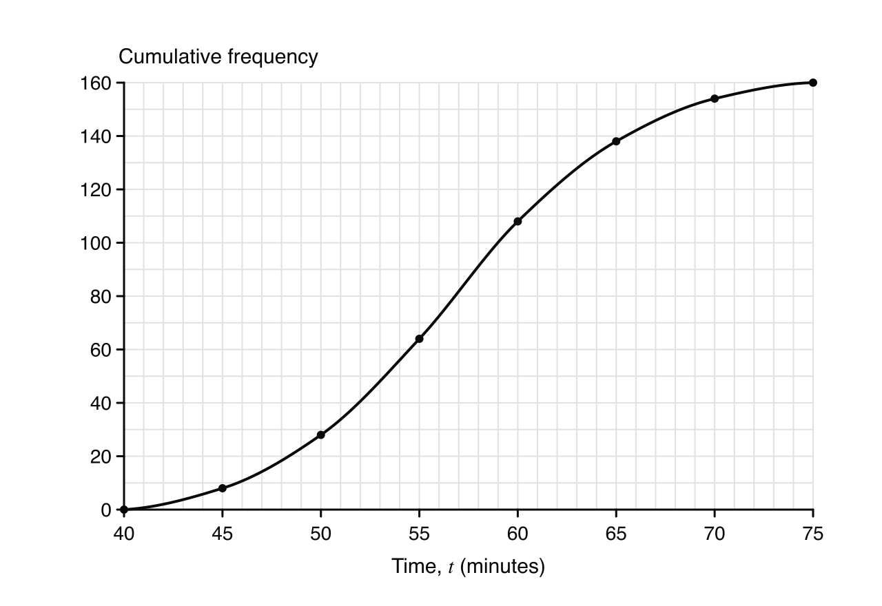
Part (d) of a question like this is where many marks are lost: the frequency of a class is the difference of two cumulative frequencies, not the cumulative frequency itself.
For questions that ask whether a claim is correct, always pair the conclusion with the reason that supports it, such as a comparison with a quartile or a fence. A conclusion with no valid reason earns no marks, even if it is right.
The ages of the members of a choir, in completed years, are grouped as 18–24, 25–39 and 40–64. Write down the class 25–39 as an inequality, and its upper class boundary. [2]
The masses, kg, of 50 parcels are grouped as follows: : 6; : 14; : 17; : 9; : 4. Construct a cumulative frequency table and find the percentage of parcels heavier than 6 kg. [3]
The numbers of goals scored by a team in 10 matches are 4, 7, 8, 8, 10, 11, 13, 15, 18, 21 (sorted). Find the median, the quartiles, the interquartile range and the range. [4]
A cumulative frequency graph of the journey times of 240 commuters passes through the points (20 minutes, 60), (30 minutes, 150) and (45 minutes, 216). Write down (a) the lower quartile; (b) the 90th percentile. (c) Find the number of commuters whose journey took more than 30 minutes. [4]
A box-and-whisker diagram of the scores of 200 students has , median 48 and . Estimate the number of students who scored (a) more than 48; (b) between 35 and 60; (c) more than 60. [3]
The values 3, 18, 20, 21, 23, 24, 26, 27, 29, 31, 45 are the waiting times, in minutes, at a clinic. Find the five-number summary, determine which values are outliers, and describe where the whiskers of the box-and-whisker diagram end. [6]
Explain why the bars of a histogram of continuous data are drawn with no gaps between them. [2]
A town has 18,400 inhabitants. On the cumulative frequency graph of their ages, the cumulative frequencies at ages 20, 40 and 60 years are 4,600, 9,800 and 14,700. Find the percentage of inhabitants aged 40 or over, and write down the class, of the form , that contains the median age. [3]
Class A's test scores have five-number summary 32, 48, 61, 70, 88 and class B's have 40, 52, 58, 63, 79. Compare the two distributions. [3]
A cumulative frequency graph starts at 20 kg and ends at 70 kg. Explain why the range of the data cannot be found exactly from the graph. [2]
, because a member aged 39 years and 11 months is still in the class; upper class boundary 40.
Cumulative frequencies 6, 20, 37, 46, 50 at upper boundaries 2, 4, 6, 8, 10. Parcels over 6 kg: , so .
Median ; lower half 4, 7, 8, 8, 10 gives
(a) is read at , so
(a) about 100 (50%); (b) about 100 (the middle 50%); (c) about 50 (25%).
: median = 6th value = 24; = median of 3, 18, 20, 21, 23 = 20; = median of 26, 27, 29, 31, 45 = 29; minimum 3, maximum 45. IQR = 9, fences
The variable is continuous, so every value between the lowest and highest boundaries belongs to some class; the classes share boundaries, so their bars meet. A gap would suggest values that cannot occur.
Aged 40 or over: , so
Class A has the higher median (61 against 58), so A scored higher on average. Class B has the smaller IQR (11 against 22) and range (39 against 56), so B's scores were more consistent. A is negatively skewed (median nearer ); B is close to symmetric.
The graph runs from the lowest class boundary to the highest, so it shows only that every value lies between 20 and 70 kg; the actual minimum and maximum lie somewhere inside the first and last classes, so the range is at most 50 kg but its exact value is unknown.
A frequency distribution lists each value or class with its frequency; . Class intervals are inequalities with no gaps, such as , and grouped statistics are estimates.
The upper class boundary is the top end of a class; for ages in completed years, "30–34" has upper boundary 35.
A histogram of continuous data has touching bars on the class intervals; with equal class widths, bar height = frequency, and the shape shows symmetry or skew.
Cumulative frequency is a running total, plotted against upper class boundaries starting from (lowest boundary, 0) and joined by an increasing curve.
From a cumulative frequency graph: median at , at , at , th percentile at ; numbers above a value are minus the reading.
measures the spread of the middle 50%; range = maximum − minimum.
A box-and-whisker diagram draws the five-number summary to scale; whiskers end at the most extreme non-outliers, outliers (beyond or
Skew is named after the long tail: positive skew has the median nearer and a longer right whisker. A symmetric box-and-whisker diagram means the data may be normally distributed.
Compare distributions by centre (median), spread (IQR or range) and shape, naming the statistic and the group and interpreting in context.
I can write class intervals as inequalities without gaps and place a boundary value in the correct class.
I can find the upper class boundary of a class, including age classes in completed years.
I can draw a histogram with equal class widths, correct boundaries and no gaps.
I can explain why bar area matters and why equal class widths let the height show the frequency.
I can build a cumulative frequency table and plot it against upper class boundaries.
I can read the median, quartiles and any percentile from a cumulative frequency graph at the correct positions.
I can find the number of values above, below or between given values from a cumulative frequency graph.
I can turn cumulative frequencies back into class frequencies.
I can find the five-number summary of a short list of data by hand and with a GDC.
I can test for outliers and draw a box-and-whisker diagram to scale with whiskers and crosses in the right places.
I can say what a box-and-whisker diagram shows and what it hides.
I can identify positive skew, negative skew and symmetry from a histogram or a box-and-whisker diagram.
I can judge from a box-and-whisker diagram whether data may be normally distributed.
I can compare two distributions using the median, IQR and shape, in context.
[1 mark]
Determine whether the minimum and the maximum are outliers.
4 marks
OR (M1)
lower boundary , upper boundary A1A1
and , so both the minimum and the maximum are outliers R1
Note: Award only for both comparisons and the conclusion. FT from their part (a).
[4 marks]
The researchers know that no person can genuinely react to the test in less than 0.1 seconds. Comment on whether each of the two outliers should be kept in the data.
2 marks
0.09 s is faster than humanly possible, so the driver probably pressed before the signal (an error); remove it R1
0.44 s is a plausible (slow) reaction time, so it is a genuine value; keep it R1
[2 marks]
Lindiwe's farm has three apple orchards. The numbers of apple trees in each orchard are shown in the following table.
Orchard | Hillside | Riverbank | Valley |
|---|---|---|---|
Number of trees | 1840 | 1150 | 1010 |
Lindiwe wants to check 80 trees for disease.
She decides to use a stratified sample. Find the number of trees she should check in each orchard.
3 marks
Explain why a stratified sample may be more suitable than a simple random sample of 80 trees.
1 mark
Lindiwe also weighs apples. State whether the mass of an apple is discrete or continuous data.
1 mark
The masses, in grams, of 12 apples picked from Riverbank are:
Find
(i) the mean mass;
(ii) the standard deviation of the masses.
3 marks
(i) Find the lower quartile, the median and the upper quartile of the masses.
(ii) Show that the mass of 236 g is an outlier.
6 marks
Draw a box-and-whisker diagram to represent the masses of the 12 apples, using a horizontal scale from 120 g to 240 g.
3 marks
Lindiwe checks her notebook and confirms that the 236 g apple was weighed correctly. State, with a reason, whether she should remove it from the data.
1 mark
The times taken by 160 runners to complete a 5 km park run are shown on the following cumulative frequency curve.
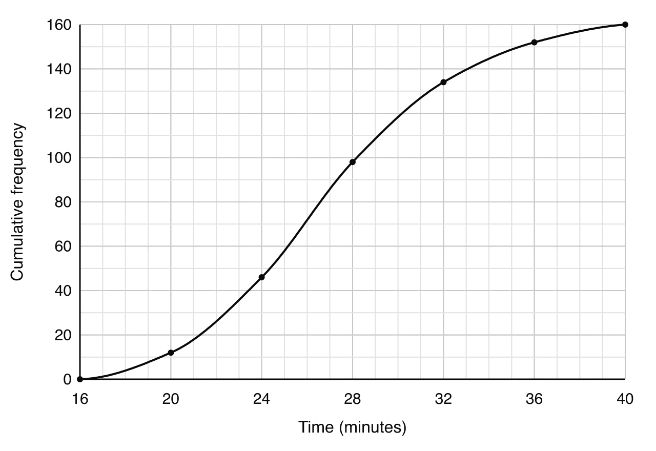
Use the cumulative frequency curve to estimate
(i) the median time;
(ii) the lower quartile;
(iii) the upper quartile;
(iv) the interquartile range.
4 marks
Estimate the number of runners who took more than 30 minutes.
2 marks
Write down the number of runners who took between 24 and 28 minutes.
1 mark
Length of call, minutes | |||||
|---|---|---|---|---|---|
Frequency | 7 | 12 | 7 | 3 | 1 |
Check: , the number of calls.
The minimum 9 is above 8, so there is no outlier at the low end. The maximum 26 is above 24, so it is an outlier. The diagram should end the right whisker at the largest value below 24 and mark 26 with a cross.
(ii) readings at 40 and 120 seen (M1)
, (accept ) (A1)
minutes (accept 9.5 to 10.3) A1
(c) (M1)
47.5 minutes (accept 47 to 48) A1
(d) A1
A1
(e) (M1)
upper fence A1
, so 74.3 is not an outlier R1
Note: Follow through from their quartiles. Do not award R1 without a comparison.
(f) median at 56.8 A1FT
box from 51.9 to 61.7 A1FT
whiskers to 41.2 and 74.3, level with the middle of the box, drawn with a ruler A1
Note: Award at most A1A1A0 if a horizontal line goes through the box.
(g) the median this year is lower (56.8 < 58.5), so runners were faster on average this year A1
the IQR this year is smaller (9.8 < 13.0), so the times were more consistent this year A1
Note: Do not accept a comparison of means.
Total [18]