4.1 Collecting data and sampling

Populations and samples

A statistical investigation begins with a question about a group: the average sleep of the students in a school, the proportion of voters who support a policy, the lifetime of the light bulbs made in a factory this month. The whole group the question is about is the population. The question fixes the population, whatever is convenient to measure: if the question asks about all students in a school, then students absent on the day of the survey are still part of the population.

Collecting data from every member of a population is called a census. A census gives the exact population value of any statistic, apart from errors in measuring and recording. Many countries run a national census every ten years, and a teacher who records the marks of every student in a class has taken a census of that class.

A census is often impossible or not worth its cost. The population may be very large (every adult in a country), spread out, constantly changing (fish in a lake), or infinite in principle (every throw of a die). Some measurements also destroy the item: testing how long a battery lasts uses it up, so a factory that tested every battery would have none left to sell. In all these cases the investigation measures a sample instead.

Statistics as estimates of population values

A number that describes a population, such as the mean height of all 16-year-olds in a country, is usually unknown. The same calculation done on a sample gives an estimate of it. Statisticians call the fixed population value a parameter and the value calculated from a sample a statistic, and they use different symbols for the two: $\mu$ for a population mean and $\bar{x}$ for a sample mean. A different sample would give a slightly different $\bar{x}$, while $\mu$ does not change.

How close the estimate is depends on two separate things: how large the sample is, and how it was chosen. A larger sample reduces the random variation from one sample to the next. It does nothing to correct a sample chosen in a way that favours some members of the population over others.

The sampling frame

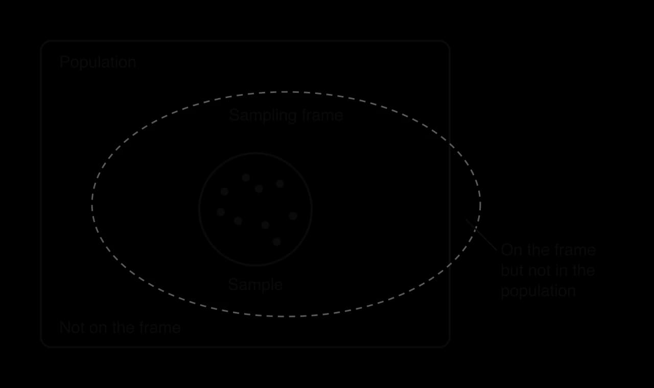
To choose a sample, an investigator needs a list or map of the population from which members can actually be selected: the school's register of students, the electoral roll, a list of the serial numbers of the bulbs made this month. That list is the sampling frame.

A perfect sampling frame lists every member of the population exactly once and nobody else. Real frames rarely do. A list of landline telephone numbers misses people who use only a mobile phone; an electoral roll includes people who have moved away and misses people who have just turned 18; a club's mailing list may still hold members who left last year. The diagram of a population and its frame shows both kinds of fault: part of the population is not on the frame and can never be chosen, and part of the frame is not in the population at all.

A sample drawn from a faulty frame inherits the frame's faults, however carefully the sample itself is chosen. This is one of the main reasons a sample can misrepresent its population, and it is the first thing to check when judging a survey.

Random samples

A sample is useful only if it is typical of the population, so that its statistics are close to the population's. The most reliable way to achieve this is to let chance decide who is chosen. When chance decides, no feature of a member (age, opinion, whether they are easy to reach) makes them more likely to be picked, so the sample has no built-in tendency to favour one kind of member.

Random does not mean haphazard. Stopping "random" people in a shopping centre is not a random sample in the statistical sense, because the people who happen to be in that place at that time, and whom the interviewer chooses to approach, are not chosen by chance from the whole population. A random sample needs a sampling frame and a chance mechanism such as a random number generator.

Types of data

Before data are collected, an investigator needs to know what kind of values they will be, because the type of data decides which graphs and calculations make sense. The first distinction is between data that are categories and data that are numbers.

Qualitative data can be counted (how many students chose each subject) and shown in bar charts or pie charts, but they cannot be averaged. Codes that look like numbers can still be qualitative: a football shirt number or a postcode is a label, and the mean of a team's shirt numbers has no meaning.

Discrete and continuous data

Quantitative data split again according to the values they can take. Counting produces separate values with gaps between them: a family can have 2 or 3 children but not 2.4. Measuring produces values on a continuous scale: a height could be 172 cm, 172.4 cm or 172.43 cm, and only the precision of the ruler stops the list of possible values.

The values of discrete data do not have to be whole numbers. Shoe sizes in steps of a half, or IB grades from 1 to 7, are discrete because only certain separate values are possible. The test is whether there are gaps between the possible values, not whether the values are integers.

Measured data are always recorded to some accuracy, so a list of continuous data can look discrete. A runner's time recorded as 15.2 s is still continuous: the true time is somewhere between 15.15 s and 15.25 s, and the rounding comes from the stopwatch, not from the quantity. Rounding to a fixed precision is a source of measurement error, taught in subtopic 1.6. Age is the classic awkward case: age in completed years is usually recorded as a whole number, but age itself is a continuous measure of time.

The type of data also decides how data are grouped and drawn. Grouped continuous data are shown in a histogram with class intervals that meet without gaps, while discrete data can be shown with separate bars; subtopic 4.2 covers both.

Reliability of data sources and bias

Data reach an investigation in one of two ways. Primary data are collected by the investigator for the purpose in hand, and secondary data were collected by someone else, often for another purpose, and are taken from a published source such as a statistics office, a sports federation or a website. Either kind can be good or bad, and the questions to ask about them are the same.

Questions to ask of any data source

Judging reliability comes down to a short list of questions. Each one points to a different way data can go wrong.

• Who collected the data, and why? A national statistics office or a peer-reviewed study has methods that others can check. A company reporting on its own product, or a campaign group reporting on its cause, may have a reason to present the data in one light.

• How were the members chosen? A random sample from a good frame can be generalised to the population; a self-selected online poll cannot.

• How large is the sample? Small samples give estimates that vary a lot from one sample to the next.

• How were the values measured or recorded? Self-reported values (a person's own estimate of their screen time) are less reliable than measured ones; different instruments or definitions give values that cannot be compared.

• When were the data collected? Prices from ten years ago, or a survey taken in one unusual week, may not describe the situation now.

• Is anything missing or obviously wrong? Blank entries, impossible values and duplicated rows are signs that the data need checking before use.

A source can be reliable in one sense and not in another. Official exchange rates published by a central bank are accurate and consistent, but if a project needs the prices that tourists actually pay at street kiosks, they are the wrong data. Reliability is always judged against the question being asked.

Bias

When a sample is chosen in a way that consistently favours some members of the population, its statistics are pulled in one direction and do not average out to the population value, however large the sample. This systematic error is called bias.

Random error and bias behave differently. Random error comes from the luck of which members happen to be chosen; it is as likely to push an estimate up as down, and it shrinks as the sample grows. Bias pushes the estimate the same way every time and does not shrink with sample size. A sample of 10 people can have large random error and no bias; a sample of 2 million can have tiny random error and a large bias.

Bias enters at several points in collecting data. The main sources, with examples of each, are listed in the table.

In 2008 Google launched Google Flu Trends, which estimated influenza activity in the United States from the number of flu-related web searches. It missed the spring 2009 pandemic and overestimated flu levels across 2011–2013, and Google stopped publishing its estimates in August 2015. Millions of searches are not a random sample of people with flu: they come from whoever chooses to search, for whatever reason, and that group changes as news coverage and the search engine itself change.

Source: Google Flu Trends, Wikipedia; Lazer et al., "The Parable of Google Flu", Science, 2014.

Missing data and errors in recording

Real data sets have gaps and mistakes. A respondent skips a question, a sensor fails for an hour, a value is typed with the decimal point in the wrong place or in the wrong units. These problems are part of the reliability of the data, and they must be found and dealt with before any statistics are calculated.

The rule for missing data is to never invent values. The honest options are to remove the incomplete record from the calculation and say so, or, if the missing value can be recovered from the original source, to recover it. Replacing a blank with 0 is especially damaging, because 0 is a real value that drags every average down.

Suppose 12 households are asked how much they spent on travel last week (in dollars), and one household leaves the answer blank.

The 11 recorded values add up to 393. Leaving out the missing value and dividing by 11 gives a mean of about $35.73, which is the right summary of the households that answered. Entering the blank as 0 and dividing by 12 gives $32.75, about $3 too low, and describes no household in the survey. A report would give the mean as $35.73 for 11 households and note that one did not respond.

Recording errors are values that were written down wrongly. Common types are values in the wrong units, a misplaced decimal point, digits typed in the wrong order, a duplicated record and a value that is impossible for the quantity (a negative mass, a percentage above 100, a person aged 250). They are found by sorting the data, looking at the largest and smallest values, and asking whether every value is possible and plausible in context.

Errors that are less extreme are harder to spot. A height recorded as 186 cm instead of 168 cm (two digits swapped) is perfectly possible, and no check on the data alone can find it. This is why careful recording at the time of collection matters more than any cleaning afterwards.

Outliers

Some values in a data set lie far from the rest. They may be recording errors, like the heights of 1.75 and 1640, or they may be genuine but unusual members of the population. Either way they deserve attention, because a single extreme value can change a mean, a standard deviation or a correlation coefficient considerably. Statistics needs a clear rule for deciding when a value is far enough from the rest to be called an outlier.

Quartiles and the interquartile range

The rule measures distance from the middle half of the data. When the data are in order, the lower quartile $Q_1$ is the value a quarter of the way through the data, and the upper quartile $Q_3$ is the value three quarters of the way through. The middle 50% of the data lie between them, and the interquartile range is the distance between them.

The IQR measures the spread of the middle half of the data, so it is not affected by a few extreme values at either end. That makes it a sensible ruler for judging how far away an extreme value is. Subtopic 4.2 explains quartiles in full, including how to read them from a cumulative frequency graph.

The 1.5 × IQR rule

A value is called an outlier when it lies more than one and a half interquartile ranges beyond the nearer quartile. The two boundary values are called fences.

Any value below the lower fence or above the upper fence is an outlier. A value exactly on a fence is not an outlier, because the definition says "more than".

The number 1.5 is a convention, proposed by the American statistician John Tukey as a practical rule for exploring data. It is chosen so that the rule rarely flags values in well-behaved data. For data that follow a normal distribution, the quartiles lie about $0.674\sigma$ either side of the mean, so the IQR is about $1.349\sigma$ and the fences are about $2.698\sigma$ from the mean.

Only about 0.7% of normally distributed values lie that far out, so in a typical bell-shaped data set fewer than 1 value in 100 is an outlier. When many values in a data set fall beyond the fences, something unusual is usually going on: the distribution is strongly skewed, the data mix two different groups, or there are errors.

Testing for outliers step by step

The test always follows the same four steps.

1. Find $Q_1$ and $Q_3$ (from the GDC's one-variable statistics, or as given in the question).

2. Calculate $\mathrm{IQR} = Q_3 - Q_1$.

3. Calculate the fence on the side of the value being tested: $Q_3 + 1.5 \times \mathrm{IQR}$ for a large value, $Q_1 - 1.5 \times \mathrm{IQR}$

4. Compare the value with the fence and state the conclusion.

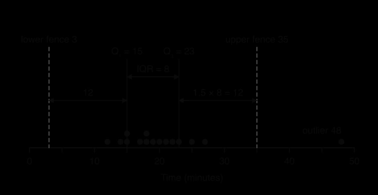
Fifteen students time how long, in minutes, they take to complete a logic puzzle.

The GDC gives $Q_1 = 15$ and $Q_3 = 23$, so the IQR is 8 and $1.5 \times 8 = 12$. The fences are $15 - 12 = 3$ and $23 + 12 = 35$. The time of 48 minutes is greater than 35, so it is an outlier; no time is below 3, so there is no low outlier. The number line of the puzzle times shows the fences 12 minutes outside each quartile and the single point beyond the upper fence.

Using the GDC to find the quartiles

Ordering raw data and calculating quartiles by hand is slow, so in practice the GDC's statistics functions do it.

1. Enter the data in a list (on a TI-84 Plus CE: STAT → EDIT; on a Casio fx-CG50: MENU → Statistics).

2. Run one-variable statistics on the list (TI-84 Plus CE: STAT → CALC → 1-Var Stats; Casio fx-CG50: CALC → 1-VAR). If the data are in a frequency table, enter the values in one list and the frequencies in another and set the frequency list.

3. Read off $Q_1$, the median and $Q_3$ from the output, together with the minimum and maximum.

Different calculators and spreadsheets use slightly different rules for quartiles. For the puzzle data, most GDCs give $Q_1 = 15$ and $Q_3 = 23$, while a common spreadsheet function gives 16 and 22.5. Quartiles quoted as GDC output use the GDC's method (the median of each half, leaving out the overall median when the number of values is odd); subtopic 4.3 compares the methods.

Finding the values that would be outliers

The fences describe a whole range of values that would count as outliers, which allows a question to work backwards: given the quartiles, what values of an unknown would be outliers? Questions of this kind need care when the unknown value could change the quartiles themselves.

Interpreting outliers

Once a value has been identified as an outlier, a judgement follows. An outlier is either a genuine member of the population that happens to be extreme, or an error in the data, and the two must be treated differently.

• A genuine outlier is a valid part of the sample and should normally be kept. Removing it would make the data describe a population without its extreme members. The tallest player in a basketball squad, a record-breaking flood or the one student who did not finish a puzzle are real values.

• An error (a value typed wrongly, measured in the wrong units, or from a member who should not be in the population) should be corrected if the true value can be found, and otherwise removed, with the removal reported.

Which of the two it is depends on the context. A body temperature recorded as 3.7 °C is impossible for a living person and is almost certainly 37 °C with the decimal point misplaced. A puzzle time of 48 minutes is unusual but possible: that student may have been interrupted, or may have found the puzzle hard. Before removing it, the investigator would ask what happened, and if the time is genuine it stays in the data.

When outliers are kept, the choice of summary matters. The median and IQR are hardly affected by an extreme value, while the mean and standard deviation can change a lot; subtopic 4.3 shows this in detail. Outliers are marked as separate crosses on a box-and-whisker diagram (subtopic 4.2), and they can distort Pearson's correlation coefficient far more than Spearman's (subtopic 4.10).

Sampling techniques

There are many ways to choose a sample, and they differ in how well the sample represents the population, how much they cost and what information they need in advance. Five techniques are in common use. Three of them (simple random, systematic and stratified) use chance to select members; two (quota and convenience) leave the choice to the person collecting the data.

Simple random sampling

The simplest way to let chance decide is to give every member of the population the same chance of selection, and to choose them independently, like drawing names from a hat.

In practice the names in a hat are replaced by numbers and a random number generator.

1. Obtain a sampling frame and number its members from 1 to $N$.

2. Use a random number generator to produce integers from 1 to $N$ (on a TI-84 Plus CE, MATH → PROB → randInt(1, N); on any GDC, the random integer function).

3. Select the members with those numbers, ignoring any number that has already been chosen, until $n$ different members have been selected.

A simple random sample has no built-in bias, and its estimates get steadily better as $n$ grows. Its weaknesses are practical. It needs a complete numbered frame, which may not exist; the chosen members may be spread out and expensive to reach; and by chance it can under-represent a small group (a random 20 students from a school might include no one from the smallest year group).

Systematic sampling

Choosing every $k$th member from an ordered list is quicker than generating many random numbers, and it spreads the sample evenly through the list.

The interval $k$ comes from the sizes of the population and the sample.

If $k$ is not a whole number, it is rounded down so that the list does not run out before $n$ members are chosen. The starting point is chosen at random from 1 to $k$; after that, every $k$th member is taken. The random start gives every member the same chance of selection, $\frac{1}{k}$, but unlike simple random sampling, most possible samples can never occur: two neighbouring members of the list can never both be chosen.

Systematic sampling suits lists and production lines: every 50th bottle from a filling machine, every 10th name on an alphabetical list, every 20th invoice. Its danger is a list with a repeating pattern that matches $k$. Taking every 7th day of a shop's daily sales records picks the same weekday every time, so the sample would describe only Tuesdays, say. If a machine has 8 filling heads and the inspector takes every 8th bottle, every bottle tested comes from the same head.

Stratified sampling

Many populations divide naturally into groups that differ from each other: year groups in a school, age bands in a country, departments in a company. If the groups differ in the quantity being studied, a sample that has the wrong mix of groups will be biased. Stratified sampling fixes the mix in advance.

The number taken from each stratum matches the stratum's share of the population. A stratum that makes up 30% of the population supplies 30% of the sample.

People cannot be split into fractions, so each result is rounded to a whole number. Rounding each value to the nearest integer usually works, but the rounded numbers must add up to the sample size. When they do not, the stratum whose number was closest to rounding the other way (the largest decimal part below 0.5 when one more is needed, the smallest above 0.5 when one fewer is needed) is adjusted.

The population of Brazil in 2023, split into three broad age bands, shows the method on a real population table. A survey company wants a stratified sample of 1,200 people.

Source: World Bank, World Development Indicators (SP.POP.0014.TO, SP.POP.1564.TO, SP.POP.65UP.TO), 2023 values, accessed 2026.

The three rounded numbers add to 1,200, so no adjustment is needed. Within each band, the 239, 833 or 128 people would then be chosen by simple random sampling. A simple random sample of 1,200 Brazilians would have the right age mix only on average; the stratified sample has it exactly, so an estimate of anything that varies with age (hours of sleep, internet use, health spending) is more precise.

Stratified sampling gives the most representative sample of the five techniques when the strata really differ. It needs more information than the others: a frame for each stratum and the size of every stratum. It also needs a sensible choice of strata, which depends on what is being studied.

Quota sampling

Market researchers and pollsters often want a sample with the right mix of groups but have no list to choose from. Quota sampling sets the number needed from each group (the quota) and lets interviewers find people until each quota is filled.

Quota sampling and stratified sampling look alike, since both fix the number from each group. The difference is how the members within each group are chosen. In stratified sampling they are chosen at random from a frame; in quota sampling the interviewer chooses them, usually whoever is available. A quota of 20 women aged 18–30 might be filled by the first 20 such women to walk past an interviewer in a city centre on a weekday morning, who are not typical of all women aged 18–30.

The quotas do not have to be proportional. An investigation might ask for 4 boys and 4 girls, or 10 students from each class, whatever the sizes of the groups. Quota sampling is quick, cheap and needs no frame, and it guarantees that every category appears. Its weakness is bias within each category, which no quota can remove.

Convenience sampling

The cheapest sample of all consists of whoever is easiest to reach.

Asking classmates, surveying shoppers outside one shop, testing every patient who visits a clinic on one day, or posting an online poll that anyone can answer are all convenience samples. A volunteer sample is a convenience sample in which members choose themselves. Convenience samples are quick and cheap and can be useful for a first look at a question or for testing a questionnaire, but the members are rarely typical of the population, so results should not be generalised.

Identifying the technique

In an investigation described in words, the technique is identified by asking how the members were chosen, step by step. The flowchart of sampling techniques gives the questions in order: random or not, then how the population was split or listed.

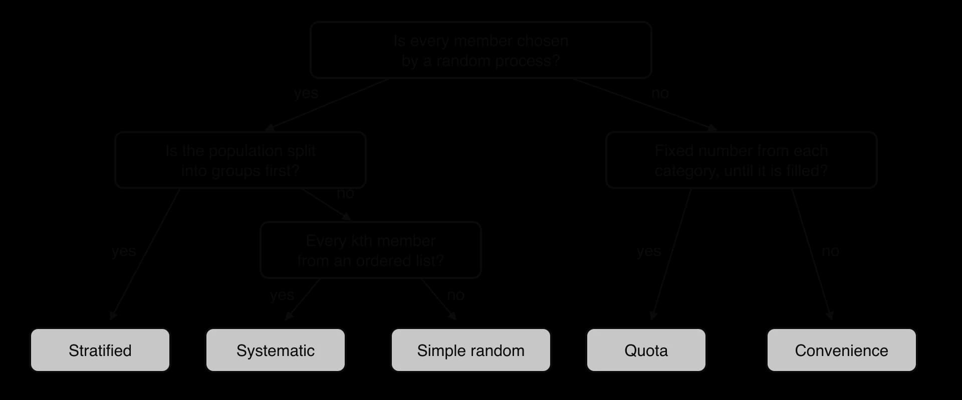
A description can fit more than one technique. A principal who asks for volunteers, then takes the first four boys and the first four girls who reply, has used quota sampling (fixed numbers per category) with members chosen by convenience. Where a single best description is needed, the more specific technique (quota) is the better name; where two are wanted, both can be named.

Comparing the techniques

No single technique is best in every situation. The choice depends on whether a frame exists, whether the population has important subgroups, and how much time and money are available.

Judging the effectiveness of a sample

A judgement about a sample should name a specific problem and say how it affects the results. "The sample is too small" on its own is weak, because a small random sample has no bias; its estimates are only less precise. Stronger comments link the problem to the population.

• The method was not random (volunteers, whoever was nearby), so certain kinds of people are likely to be over-represented.

• The frame leaves out part of the population, so those members could never be chosen.

• Many people did not respond, and those who did may differ from those who did not.

• The sample came from one place or one time (one class, one city, one day), so it may not represent the whole population.

• The quotas or strata do not match the population's real proportions.

A sample can also be fine for one question and poor for another. Patients at a clinic on one day are a reasonable sample of that clinic's patients, but not of the whole town, because healthy people are not at the clinic.

Case study: the 1936 Literary Digest poll

In 1936 the United States held a presidential election between the Democratic president Franklin D. Roosevelt and the Republican Alf Landon. The magazine The Literary Digest ran one of the largest opinion polls ever attempted. It mailed about 10 million ballots, using its own readers and lists of car owners and telephone users as the sampling frame, and about 2.38 million were returned. It predicted that Landon would win with 57.08% of the popular vote.

At the same time George Gallup, who had begun running scientific polls, predicted a Roosevelt victory from a quota sample of 50,000 people chosen to match the make-up of the electorate.

Source: "The Literary Digest" and "1936 United States presidential election", Wikipedia, accessed 2026.

What went wrong

The response rate was

so more than three-quarters of those mailed did not reply. The errors of the two polls can be compared directly.

The Digest put Landon comfortably ahead, yet Roosevelt won by more than 24 points and carried 46 of the 48 states. Gallup's estimate was also about 5 points out, but its error was about a quarter of the Digest's and it named the right winner.

Two kinds of bias combined. The sampling frame was biased: in the middle of the Great Depression, people who subscribed to a magazine, owned a car or had a telephone were wealthier than average, and wealthier voters were more likely to support Landon. Later research concluded that non-response bias was the larger cause: Landon's supporters were more likely than Roosevelt's to send their ballots back. Neither bias got smaller as more ballots arrived, because every extra reply came from the same biased frame and the same self-selected group.

What the case shows

Gallup's 50,000 people were about one-fiftieth of the Digest's 2.38 million replies.

The smaller sample won because it was designed to match the population. With a random or well-designed sample, the random error in an estimated proportion from 50,000 people is well under one percentage point, so the Digest's error came from bias, not from too few replies.

Gallup's method had weaknesses too. In 1948 the major polls, Gallup's among them, wrongly predicted that Thomas Dewey would defeat Harry Truman. A quota sample still leaves the choice of people within each category to interviewers, which can bring bias back in; choosing at random within each category, the idea behind stratified sampling, removes that choice. The Literary Digest itself folded within 18 months of the 1936 election.

Exam focus

Collecting data and sampling usually appears as the opening parts of a longer statistics question on Paper 1 or Paper 2, worth 1–4 marks, before the question moves on to box-and-whisker diagrams, correlation or a hypothesis test. The command terms are mostly state, identify, name and write down for sampling techniques and data types (one mark each, no working needed), calculate for stratified sample sizes, and determine, show that or justify for outlier tests. Explain, suggest and comment appear when a question asks why a sample may not represent the population or why a prediction differed from what happened.

Outlier tests are the most frequent calculation. A typical markscheme gives (M1) for $Q_3 + 1.5 \times \mathrm{IQR}$ or $Q_1 - 1.5 \times \mathrm{IQR}$ seen with numbers, A1 for the fence value, R1 for comparing the data value with the fence, and A1 (or AG in a "show that") for the conclusion; the R1 depends on the method, and a conclusion without the comparison earns nothing. Sampling-technique answers earn A1 only for the exact name, and questions that ask for two techniques give A1A0 for one right and one wrong. HL Paper 3 questions often use the same ideas to criticise how a study's data were collected.

The examples of a fastest time just inside its fence (13.9 against 13.8) and a slowest time outside its fence show why the inequality must be written out: the two values look equally extreme, but only one is an outlier.

Questions often describe a method in a paragraph and ask for the technique. Read for the two details that decide it: whether chance chose the members, and whether a fixed number was required from each group.

Practice questions

1. A researcher measures the number of eggs laid each week by the hens on a farm, and the mass of each egg. State whether each set of data is discrete or continuous. [2]

2. A factory makes 6,000 light bulbs a day. A quality controller tests 60 bulbs a day by running them until they fail. (a) Identify the population and the sample. (b) Explain why a census is not suitable. [3]

3. For a data set, $Q_1 = 42$ and $Q_3 = 58$. Determine whether the values 17 and 81 are outliers. [4]

4. A school has 760 students: 168 in Grade 8, 174 in Grade 9, 151 in Grade 10, 139 in Grade 11 and 128 in Grade 12. Find the number of students from each grade in a stratified sample of 40. [3]

5. A list of 4,500 members of a gym is in alphabetical order. A systematic sample of 90 is required. (a) Find the sampling interval. (b) The random start is 23. Write down the numbers of the 2nd and the last member chosen. [3]

6. For each method, identify the sampling technique. (a) A teacher asks for volunteers and takes the first 5 from each of her four classes. (b) A manager chooses 12 employees by drawing their staff numbers from a bag containing every staff number. (c) A reporter interviews shoppers outside one supermarket on a Monday morning. [3]

7. A survey website invites visitors to vote on whether school uniforms should be abolished; 84% of the 12,000 votes say yes. Explain why this result may not represent the views of all students. [2]

8. A data set of 7 values in order is 3, 5, 6, 8, 9, 11, $x$, where $x \ge 11$. Using $Q_1$ as the 2nd value and $Q_3$

9. A doctor records a patient's temperature on 15 mornings. The GDC gives $Q_1 = 36.6$ °C and $Q_3 = 36.9$ °C. One reading is 3.68 °C. (a) Show that 3.68 is an outlier. (b) Suggest what should be done with this reading. [4]

10. Explain the difference between stratified sampling and quota sampling, and suggest why stratified sampling usually gives a more representative sample. [3]

Summary

• The population is the whole group an investigation is about; a census measures every member, and a sample is the subset actually measured. Sample statistics such as $\bar{x}$ estimate population values such as $\mu$.

• At SL a data set is treated as the population unless a question says otherwise, so the GDC's $\sigma_x$ is used.

• The sampling frame is the list a sample is chosen from; members missing from the frame can never be chosen.

• Qualitative data are categories; quantitative data are numbers. Discrete data are counted and take separate values; continuous data are measured and can take any value in an interval, even when rounded.

• Reliable data come from a clear, checkable method. Bias is a systematic error from selection, non-response, self-selection, responses or measurement, and a larger sample does not remove it.

• Missing data are never invented: exclude the record and report it, or recover the true value. Recording errors are corrected from the source or removed, with the removal reported.

• $x$ is an outlier if $x < Q_1 - 1.5 \times \mathrm{IQR}$ or $x > Q_3 + 1.5 \times \mathrm{IQR}$

• A genuine outlier is a valid part of the data; an outlier caused by an error is corrected or removed.

• Simple random, systematic and stratified sampling select members by chance; quota and convenience sampling do not. Stratified numbers are $\frac{\text{stratum size}}{\text{population size}} \times \text{sample size}$, rounded to whole numbers that add up to the sample size.

• A well-designed small sample can be far more accurate than a huge biased one, as the 1936 Literary Digest poll showed.

Self-check

• To do:

  I can identify the population, sample and sampling frame in a described investigation.

• To do:

  I can explain why a census is sometimes impossible or unsuitable.

• To do:

  I can explain the difference between a sample statistic and the population value it estimates.

• To do:

  I can classify data as qualitative or quantitative, and quantitative data as discrete or continuous, even when measured values are rounded.

• To do:

  I can list questions to ask about the reliability of a data source.

• To do:

  I can name and explain at least four sources of bias, and explain why a larger sample does not remove bias.

• To do:

  I can deal with missing values and recording errors without inventing data.

• To do:

  I can find $Q_1$ and $Q_3$ with my GDC's one-variable statistics.

• To do:

  I can calculate both outlier fences and write a complete outlier test with the inequality and the conclusion.

• To do:

  I can find the values of an unknown that would make it an outlier.

• To do:

  I can judge in context whether an outlier is a genuine value or an error, and what to do with it.

• To do:

  I can describe each of the five sampling techniques and identify which one a description uses.

• To do:

  I can calculate a stratified sample and adjust the rounding so the total is correct.

• To do:

  I can find the sampling interval and the selected members in a systematic sample.

• To do:

  I can comment on the effectiveness of a sample with a specific reason linked to the population.

(b) $\mathrm{IQR} = 47 - 35 = 12$, so

$x$ is an outlier when $x > 65$. A value of exactly 65 is not an outlier, so the smallest integer value is $x = 66$.

With 11 values, the GDC's quartile method and the method of taking the $\frac{n+1}{4}$th and $\frac{3(n+1)}{4}$th values agree (3rd and 9th values), so the answer does not depend on the calculator.

$64 < 123.5$, so 64 is an outlier.

(b) $\text{upper fence} = 221 + 58.5 = 279.5$

$268 < 279.5$, so 268 is not an outlier.

(c) The value 64 is genuine (it really was the day's sales), but it comes from a day when the café was open for only half the day, so it does not describe a typical day of trading. For an estimate of typical daily sales it is reasonable to exclude it and report that one half-day was left out. Alternatively, keep it and use the median, which is hardly affected by one extreme value.