4.14 Linear transformations of random variables

Learning objectives

• Find the expected value, variance and standard deviation of a linear transformation $aX + b$ of a random variable.

• Calculate the expected value of a linear combination of random variables, whether or not they are independent.

• Calculate the variance of a linear combination of independent random variables, squaring each coefficient and adding.

• Distinguish between the sum of $n$ independent observations $X_1 + X_2 + \dots + X_n$ and the multiple $nX$ of one observation.

• Find probabilities for sums and differences of independent normal random variables, using technology.

• Explain the difference between a population parameter, a statistic, an estimator and an estimate, and what makes an estimator unbiased.

• Calculate the unbiased estimates $\bar{x}$ of $\mu$ and $s_{n-1}^2$ of $\sigma^2$

• Convert between $s_n$ and $s_{n-1}$ using the factor $\frac{n}{n-1}$

Introduction

Many quantities of interest are built from other random quantities. A taxi fare is a fixed charge plus a rate times a random distance; the total weight in an aircraft is the sum of many passengers' weights; the profit on a trade is the difference between two random prices. Knowing the mean and the spread of each part is enough to find the mean and the spread of the whole, provided the parts are combined linearly and, for the spread, provided they are independent. The same rules explain why the average of a sample is a trustworthy guide to the average of a population, and why the spread of a sample has to be adjusted before it is used to estimate the spread of a population.

The rules come in two parts. Means scale, shift, add and subtract in the same way as the quantities themselves. Variances follow three different rules: a shift leaves them unchanged, a scale factor is squared, and when independent quantities are combined their variances always add, even when the quantities are subtracted. Most errors with combinations of random variables come from forgetting one of these three rules.

Variance and standard deviation of a random variable

A random variable $X$ has an expected value $\mathrm{E}(X)$, its long-run mean, often written $\mu$. Two random variables can have the same expected value and behave very differently: one may always land close to its mean while the other swings far above and below it. A measure of spread is needed, and it is built the same way as the variance of a data set in subtopic 4.3: take the deviation from the mean, square it so that positive and negative deviations do not cancel, and average.

The variance is in squared units: if $X$ is a mass in grams, $\mathrm{Var}(X)$ is in $\text{g}^2$. Its square root returns to the original units and is easier to interpret.

For a fair six-sided die, the score $X$ takes the values 1 to 6 with probability $\frac{1}{6}$ each, so $\mathrm{E}(X) = 3.5$. The squared deviations from 3.5 are 6.25, 2.25, 0.25, 0.25, 2.25 and 6.25, and their mean is

so the standard deviation is $\sqrt{35/12} \approx 1.71$. For most named distributions the variance is known without any calculation: $np(1-p)$ for the

Linear transformation of a single random variable

A linear transformation changes every value of $X$ by the same rule $Y = aX + b$: multiply by a constant $a$, then add a constant $b$. Converting units, adding a fixed charge, applying an exchange rate and rescaling test scores are all linear transformations.

The expected value of aX + b

If every value of $X$ is multiplied by $a$, the long-run average is multiplied by $a$. If $b$ is then added to every value, the long-run average rises by exactly $b$. For a discrete variable this follows in one line from the definition of expected value and the fact that the probabilities add to 1:

The variance of aX + b

Adding $b$ moves every value and the mean by the same amount, so every deviation $x - \mu$ is unchanged and the spread does not change. Multiplying by $a$ multiplies every deviation by $a$, so every squared deviation is multiplied by $a^2$

The absolute value matters when $a$ is negative. The variable $Y = 100 - 5X$ has $a = -5$: it decreases when $X$ increases, but its values are just as spread out as those of $5X$

The same rules hold for data: subtopic 4.3 shows that adding a constant to every data value shifts the mean but not the standard deviation, and multiplying scales both. The random-variable version is used when the quantity is a model of a process rather than a list of observed values.

A fixed charge plus a rate per unit is one of the commonest linear transformations. The fixed part moves the mean but leaves the spread alone, while the rate scales both the mean and the standard deviation.

Rescaling to a target mean and standard deviation

Test designers, universities and competitions often rescale raw scores so that the new scores have a chosen mean and standard deviation. If raw scores $X$ have mean $\mu$ and standard deviation $\sigma$, the transformation $Y = aX + b$ with $a > 0$

Linear combinations of random variables

A linear combination adds or subtracts several random variables, each multiplied by a constant. The total mass of a suitcase and the items packed in it, the difference between the times of two runners, and the value of an investment split between two assets are all linear combinations.

Expected value of a linear combination

The mean of a sum is the sum of the means. If one shop takes $500 a day on average and another takes $300, together they take $800 a day on average, whatever the connection between them. Scaling and subtracting work in the same way, so for any random variables the expected value follows the coefficients and signs.

This result does not need the variables to be independent. Even if two shops' takings rise and fall together (both busy on sunny days), their combined mean is still the sum of their separate means; independence matters only when the spread is combined.

Independent random variables

Two random variables are independent when knowing the value of one tells nothing about the other. The idea is the same as independent events in subtopic 4.6, applied to every possible pair of values.

In models, independence is usually an assumption that has to be stated and judged. Service times of different customers, masses of different items from a production line and weights of different passengers are normally treated as independent. The masses of two cakes cut from the same sheet, the times of two runners in the same race on a windy day, or the returns on two shares in the same industry are not, and a model that assumes independence will misjudge their spread.

Variance of a combination of independent random variables

Variances of independent variables add. For two dice, the total $X_1 + X_2$ has 36 equally likely outcomes, and the variance of the totals can be found from the table of the 11 possible values. Working it through gives

The reason is that independent deviations do not systematically cancel or reinforce each other. Sometimes both dice are above average, sometimes both are below, sometimes one is above and the other below; these cases balance out so that the mixed terms average to zero, and only the separate spreads remain. The same argument works for a difference. The difference $X_1 - X_2$ of two dice runs from $-5$ to 5, a range of 10, just like the total, which runs from 2 to 12. Subtracting a random quantity adds uncertainty just as adding one does, so

Combining this with the rule $\mathrm{Var}(aX) = a^2\mathrm{Var}(X)$ for each term gives the general result for independent variables:

Every coefficient is squared, and every term is added, whatever the sign in front of it, because $(-a)^2 = a^2$.

The graph of the four normal curves shows both rules at once. The means combine with the signs ($30 + 20 = 50$ and $30 - 20 = 10$), while the variances add in both cases, so the curves for $X + Y$ and $X - Y$

YouTube

Why the variance rule needs independence

The expectation rule holds for any variables, but the variance rule can fail badly without independence. Taking $Y = X$, the most dependent case possible, gives $X + Y = 2X$, whose variance is $4\,\mathrm{Var}(X)$, not $\mathrm{Var}(X) + \mathrm{Var}(X) = 2\,\mathrm{Var}(X)$

Sums of independent observations and multiples

Two expressions look alike but describe different situations:

• $X_1 + X_2 + \dots + X_n$

Both have the same mean, $n\mu$. Their variances differ:

The total of separate observations is less spread out because high and low values tend to offset each other. A single value multiplied by $n$ has no chance to offset: if it is high, all $n$ copies are high together.

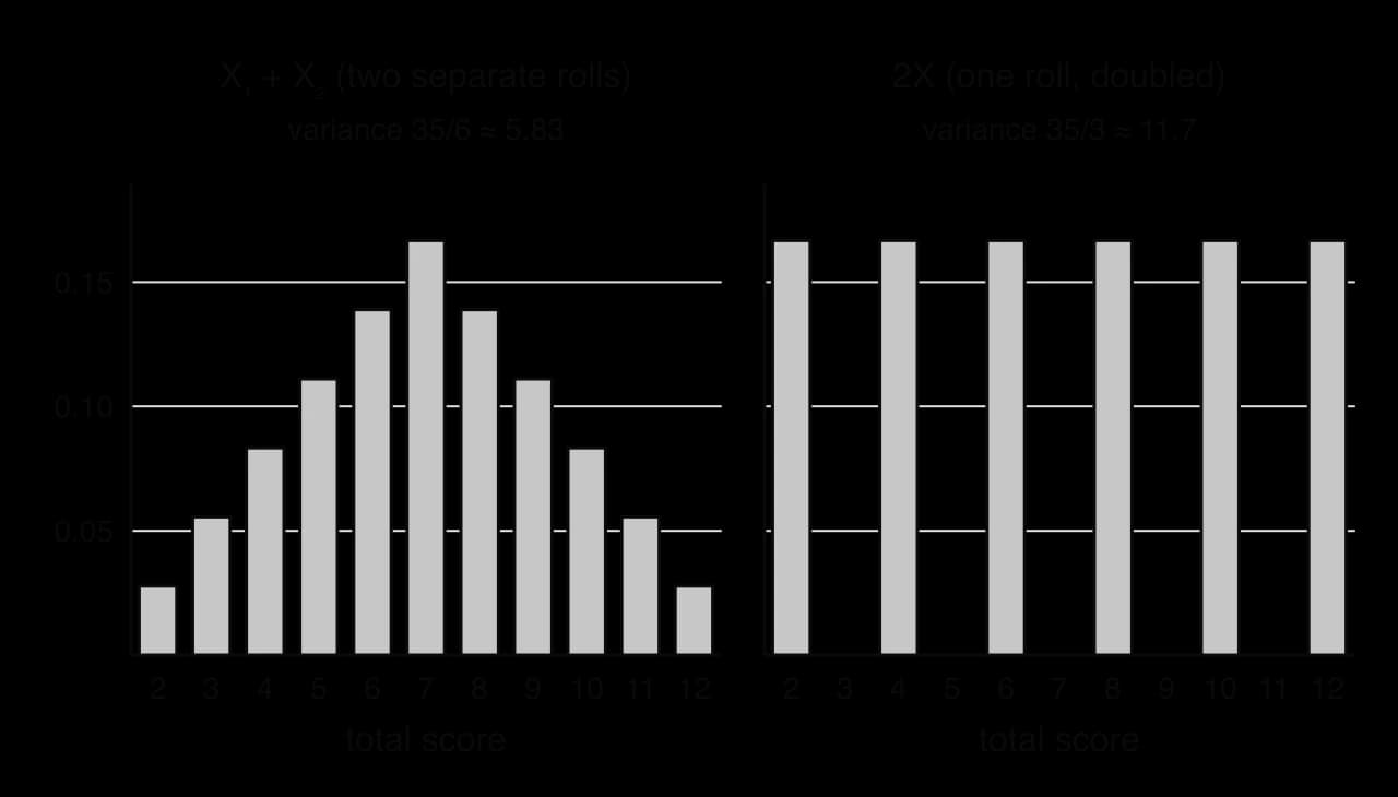
The bar charts of two dice make the difference visible. The total of two separate rolls reaches 2 or 12 only when both dice are extreme, with probability $\frac{1}{36}$ each, and is most likely to be 7. One roll doubled is equally likely to be 2, 4, 6, 8, 10 or 12, so extreme values are six times as likely. Its variance is $2^2 \times \frac{35}{12} = \frac{35}{3}$

Differences between totals

Many questions compare one quantity with a combination of others: "is one large bottle heavier than two small ones?", "does a queue of four customers clear before a queue of three?". The method is always to form a single combined variable whose sign answers the question, find its mean and variance, and then find the probability that it is positive or negative.

Variance and diversification

Combinations with coefficients other than 1 arise when a quantity is split into parts. An investor who puts a fraction $w$ of a sum into asset A, with percentage return $X$, and the rest into asset B, with return $Y$, receives the return $R = wX + (1 - w)Y$

Case study: Air Midwest Flight 5481 and the weight of passengers

On 8 January 2003, Air Midwest Flight 5481, a Beechcraft 1900D, crashed shortly after take-off from Charlotte, North Carolina, killing all 19 passengers and both crew. The loading had been calculated with the approved average passenger weights, which had not been revised since 1936. Investigators found that the real average passenger was more than 20 lb (9 kg) heavier than the estimate, and that the aircraft was 580 lb (264 kg) over its maximum take-off weight, with its centre of gravity behind the allowed limit. A maintenance error in the elevator controls also contributed.

Source: Wikipedia, "Air Midwest Flight 5481", summarising the US National Transportation Safety Board report; accessed 2026.

A total load is a sum of independent random variables, so the rules for linear combinations show what goes wrong when the mean used for planning is too low. The model below is hypothetical: suppose the weight of an adult passenger with carry-on bags, $W$ kg, has mean 91 kg and standard deviation 15 kg, while the loading sheet assumes 82 kg per passenger, 9 kg too low. For 19 passengers, the total is $T = W_1 + W_2 + \dots + W_{19}$

The loading sheet expects $19 \times 82 = 1558$ kg. The planning error grows in proportion to the number of passengers, $19 \times 9 = 171$ kg, while the random variation of the total grows only with $\sqrt{19}$

With a correct planning figure, random variation alone pushes the real load more than 100 kg over the plan on only about 6% of flights, and a safety margin can be set to cover that. With a planning figure 9 kg too low, the same overload happens on about 86% of flights. Random variation in a sum of many independent parts partly cancels out, whereas an error in the assumed mean is repeated for every passenger and builds up in full. A consistent error of this kind is a bias, and avoiding bias is the main requirement when a mean or a variance is estimated from a sample.

Population parameters, statistics and estimators

Statistical work usually runs in the opposite direction. Instead of knowing $\mu$ and $\sigma^2$ and predicting a total, a researcher has a sample and wants to learn about the population it came from. The numbers that describe the population are fixed but unknown; the numbers calculated from the sample are known but change from sample to sample.

The word "parameter" here has the statistical meaning; it is a special case of a parameter of a model, the constant that fixes which member of a family of distributions is used.

A statistic used to guess a parameter is called an estimator. The distinction between the rule and the number it produces matters: the rule "add the values and divide by $n$" is the same for every sample, while the number it gives changes each time.

The sample mean $\bar{X} = \frac{X_1 + X_2 + \dots + X_n}{n}$

Unbiased and biased estimators

Different samples give different estimates, so any single estimate will usually miss the true value. A good estimator should at least be right on average: if it were applied to every possible sample, the mean of all its estimates should equal the parameter.

An unbiased estimator can still be far from the truth for an unlucky sample. Unbiasedness describes the average behaviour of the method and gives no guarantee about any single estimate.

The bias of a sample in subtopic 4.1 comes from how the sample is chosen; the bias of an estimator comes from the formula applied to it. Both push results consistently in one direction, and neither is reduced by taking a larger sample of the same kind.

The sample mean as an unbiased estimate of μ

The sample mean is the obvious estimator of a population mean, and it is unbiased. The calculation is the formula for the mean of data from subtopic 4.3, $\bar{x} = \frac{\sum x_i}{n}$, or $\bar{x} = \frac{\sum f_i x_i}{n}$

The rules for linear combinations show why it is unbiased. Each observation $X_i$ of a random sample has mean $\mu$, and $\bar{X}$ is the linear combination $\frac{1}{n}X_1 + \frac{1}{n}X_2 + \dots + \frac{1}{n}X_n$

The same rules give the spread of $\bar{X}$ when the observations are independent: $\mathrm{Var}(\bar{X}) = n \times \frac{1}{n^2}\sigma^2 = \frac{\sigma^2}{n}$

The unbiased estimate of the population variance

Estimating $\sigma^2$ is less straightforward. The natural choice is the variance of the sample, dividing by $n$, written $s_n^2$:

This is a biased estimator: on average it is too small. The deviations are measured from $\bar{x}$, the centre of the sample itself, rather than from the unknown $\mu$. The sample mean is always the point that makes the sum of squared deviations of that sample as small as possible, so measuring from $\bar{x}$ gives a smaller total than measuring from $\mu$ would, except in the rare case $\bar{x} = \mu$

A small population that shows the bias

The bias can be seen exactly in a tiny example. A population consists of the three values 1, 4 and 7 in equal proportions, so $\mu = 4$ and $\sigma^2 = \frac{9 + 0 + 9}{3} = 6$

The mean of the nine sample means is exactly $\mu = 4$, so $\bar{x}$ is unbiased. The mean of the nine values of $s_n^2$ is 3, only half of $\sigma^2 = 6$

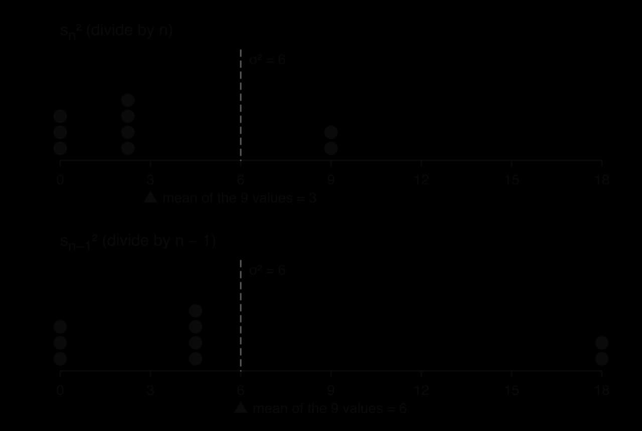
The dot plots show both estimators side by side. Neither ever gives exactly 6 for a sample of two, and $s_{n-1}^2$ is more spread out, but only $s_{n-1}^2$ is centred on the true value.

Bessel's correction

In general, $\mathrm{E}(s_n^2) = \frac{n-1}{n}\sigma^2$

One way to see why $n - 1$ is right: once $\bar{x}$ is known, the $n$ deviations $x_i - \bar{x}$

YouTube

The correction matters most for small samples. For $n = 3$ it multiplies the variance by 1.5; for $n = 10$ by about 1.11; for $n = 100$ by about 1.01. For very large samples $s_n^2$

Estimates from raw data with a GDC

A GDC's one-variable statistics function gives both standard deviations at once. The labels differ between models, which causes many errors.

On a TI-84 Plus CE, enter the data in a list and use STAT → CALC → 1-Var Stats; on a Casio fx-CG50, use MENU → Statistics → CALC → 1-VAR. The GDC gives $s_{n-1}$, a standard deviation; the unbiased estimate of the variance is its square.

Estimates from a frequency table

When data come as a frequency table, the GDC must be told the frequencies as well as the values. Without the frequency list it treats each distinct value as a single observation.

A librarian records the number of books, $x$, borrowed by each of a random sample of 50 visitors.

Estimates from the sums of x and x²

Data are sometimes summarised only by $n$, $\sum x$ and $\sum x^2$. Expanding the sum of squared deviations gives $\sum (x - \bar{x})^2 = \sum x^2 - \frac{(\sum x)^2}{n}$

An equivalent route is $s_n^2 = \frac{\sum x^2}{n} - \bar{x}^2$

Exam focus

Linear transformations, combinations and unbiased estimates appear on Papers 1, 2 and 3, often combined with the normal distribution (subtopic 4.9), the distribution of a sample mean (subtopic 4.15), or a confidence interval or test (subtopics 4.16 and 4.18) that uses the estimates found in an earlier part. Typical questions:

• find $\mathrm{E}$ and $\mathrm{Var}$ of a combination such as $2X + 7Y$ or $4X - 3Y$, sometimes for Poisson variables where the variance equals the mean (2–3 marks);

• find the probability that a total exceeds a limit, or that one quantity exceeds a multiple or a total of others, with normal variables (4–6 marks);

Marks go to: naming the combined variable; the mean; the variance with squared coefficients and added variances; the distribution with both parameters; the probability. Answers are exact or to 3 significant figures.

Questions on unbiased estimates are often the first two parts of a longer question; the answers are then used to build a confidence interval or carry out a test. Carry the unrounded values forward from the GDC, and remember that a later $t$-interval or $t$-test uses $s_{n-1}$, the square root of the unbiased variance.

Practice questions

1. A random variable $X$ has $\mathrm{E}(X) = 5$ and $\mathrm{Var}(X) = 2$. Find $\mathrm{E}(4X - 3)$

Find unbiased estimates of the population mean and variance. [3]

8. For a random sample of 12 values, $\sum x = 612$ and $\sum x^2 = 31\,540$. Find unbiased estimates of $\mu$ and $\sigma^2$

Summary

• $\mathrm{E}(aX + b) = a\mathrm{E}(X) + b$ and $\mathrm{Var}(aX + b) = a^2\mathrm{Var}(X)$

Self-check

• To do:

  I can find the mean, variance and standard deviation of $aX + b$, including when $a$ is negative.

• To do:

  I can explain why adding a constant does not change a variance.

• To do:

  I can find $a$ and $b$ to rescale a variable to a given mean and standard deviation.

• To do:

  I can find the expected value of any linear combination and know that it needs no independence.