4.13 Non-linear regression

Learning objectives

• Find the equation of a least squares regression curve (quadratic, cubic, exponential, power or sine) using technology, written in the variables of the context.

• Calculate residuals and the sum of square residuals $SS_{res}$ for a given model.

• Compare two models fitted to the same data using $SS_{res}$.

• Write down the coefficient of determination $R^2$ from technology and interpret it as the proportion of the variation in the dependent variable explained by the model.

• Explain the connection $R^2 = r^2$ for a linear model, and compare $R^2$ for a curve with $r$ for a regression line.

• Use a model to make predictions, and comment on their reliability, including extrapolation.

• Justify the choice of model using the context, the shape of the data and the residuals, explaining why $R^2$ alone is not enough.

Introduction

Many relationships in science, economics and everyday life are curved. Stopping distance grows faster than speed, air pressure falls by a constant factor for each kilometre of height, and the area of Arctic sea ice rises and falls with the seasons. A regression line cannot describe any of these well. Non-linear regression extends the least squares idea of subtopic 4.4 from straight lines to curves, so that the best curve of a chosen type can be found for any data set.

Fitting a curve with technology takes seconds. The mathematics lies in choosing which type of curve to fit, measuring how well it fits, and deciding whether a better-fitting curve is actually a better model. Two measures of fit are used for the second task: the sum of square residuals, which measures the total size of the errors, and the coefficient of determination $R^2$, which measures the proportion of the variation in the data that the model explains.

YouTube

Regression with non-linear functions

A mathematical model chosen to describe data has a fixed form, such as $y = ax^2 + bx + c$, and parameters $a$, $b$, $c$

The six families of model in the course are summarised in the table. Each family has its own shape, and the shape of the scatter diagram together with what is known about the context decides which families are worth trying.

Regression models found with the GDC. The letters are the model's parameters.

Quadratic and cubic regression

A quadratic model has one turning point and changes gradient at a constant rate. It suits quantities that rise and then fall (the height of a thrown ball, the profit at different prices) or that grow increasingly fast from a starting value, such as stopping distance.

A cubic model can have two turning points and a point of inflexion, which lets it follow an S-shaped or wave-shaped pattern over a limited range. It is used for cross-sections of rivers and roads, volumes and the shapes of objects.

Polynomial models become unreliable quickly outside the data. Every quadratic and cubic eventually heads towards $+\infty$ or $-\infty$, so predictions beyond the data range can become negative, enormous or turn in the wrong direction even when the fit inside the range is excellent.

The depth of a river is measured at 2 m intervals across its width, from one bank to the other.

Depths across a river (hypothetical data).

Exponential regression

An exponential model describes a quantity that changes by the same percentage in each equal step of $x$, the continuous version of a geometric sequence from subtopic 1.3. It is the natural model for exponential growth and exponential decay.

The two forms are the same model. Since $b^x = \mathrm{e}^{x\ln b}$, the constants are linked by

Many GDCs give $y = ab^x$. When the form $a\mathrm{e}^{kx}$ is needed, take $k = \ln b$

Power regression

A power model $y = ax^b$ passes through the origin when $b > 0$, and describes quantities in which multiplying $x$ by a factor multiplies $y$ by a fixed factor: doubling $x$

The value of $b$ often has a meaning. For a pendulum, physics predicts that the period is proportional to the square root of the length, so power regression on measured data should give $b \approx 0.5$. A value close to the predicted exponent is evidence that the theory fits.

Sine regression

A sinusoidal model describes a quantity that repeats in a regular cycle. Sine regression fits all four parameters at once.

The GDC must be in radian mode for sine regression, and the period of the fitted model is $\frac{2\pi}{b}$. Sine regression needs data covering at least one full cycle, and some GDCs accept an estimate of the period, which helps the calculation settle on a sensible answer.

Choosing which models to try

A model is chosen for reasons, and the reasons come in a definite order.

1. The context. Physical laws, growth processes and cycles suggest a family before any data are seen: populations with unlimited resources grow exponentially, seasonal quantities repeat every 12 months, braking distance depends on the square of speed.

2. The scatter diagram. The shape of the data (curving up or down, one or two turning points, a repeating pattern, levelling off) rules families in or out.

3. Behaviour outside the data. A model used for prediction must behave sensibly beyond the observed range: an exponential model of a population eventually exceeds any limit, a quadratic for a falling object eventually rises again.

4. The measures of fit, $SS_{res}$ and $R^2$, compare the candidates that survive the first three tests.

Residuals and the least squares principle

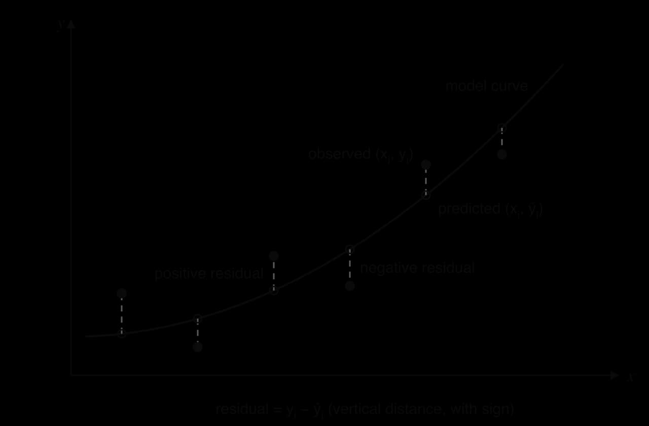
Every model gives a predicted value $\hat{y}_i$ (read "y-hat") for each data value $x_i$. The difference between what was observed and what was predicted measures how far that point is from the model.

The diagram of residuals shows them as vertical segments between each data point and the model curve. They are vertical because the model is used to predict $y$ from $x$, so its errors are errors in $y$.

The sum of square residuals

Adding the residuals does not measure the total error, because positive and negative residuals cancel: a curve that misses badly above and below can have residuals adding to zero. Squaring each residual makes every term positive and gives large misses more weight than small ones, for the same reasons as in the least squares line of subtopic 4.4.

$SS_{res}$ is zero only when the model passes through every point. Its units are the square of the units of $y$, so it can be used to compare different models fitted to the same data, but not to compare models of different data sets: a data set measured in metres and the same data in centimetres have values of $SS_{res}$

Least squares regression curves

Within one family of curves, different parameter values give different values of $SS_{res}$. The best curve of that family is the one with the smallest.

The least squares regression line of subtopic 4.4 is the special case for the linear family. For every family in the course, the GDC finds the parameters numerically. The least squares principle also gives a way to judge any model: a model chosen by some other method (from two data points, from a theory, from a graph drawn by eye) always has an $SS_{res}$ at least as large as the least squares curve of its family, and comparing the two shows how much better the fit could be.

Calculating SS_res for a given model

Models are often proposed with stated parameters, from theory or from a few data points, and two such models can be compared on the same data. The method is the same every time.

1. Use the model to calculate the predicted value $\hat{y}_i$ at each data value $x_i$.

2. Find each residual $y_i - \hat{y}_i$

On the GDC, the lists do the work: enter the $x$-values in L1 and the $y$-values in L2, define L3 as the model applied to L1 (for example $50 \times 1.5^{\text{L1}}$), define L4 as $(\text{L2} - \text{L3})^2$

Bacteria counts in a culture (hypothetical data).

The method is the same for any data set: the model with the smaller $SS_{res}$ on the same data fits better. The exponential regression on these counts gives $N = 52.5 \times 1.49^t$, whose sum of square residuals is about 21.6, so even Model A is far from the best exponential fit.

Finding regression curves with technology

All the least squares curves in the course come from the GDC's statistics menu. The procedure is the same for every family; only the regression type changes.

1. Enter the independent variable in one list and the dependent variable in another.

2. Draw a scatter diagram to see the shape.

3. Choose the regression type: on a TI-84 Plus CE, STAT → CALC → QuadReg, CubicReg, ExpReg, PwrReg or SinReg; on a Casio fx-CG50, MENU → Statistics → CALC → REG, then the type (X^2, X^3, Exp, Pwr, Sin).

4. Read the parameters and, where shown, $R^2$. On a TI-84 Plus CE, $R^2$ appears only if DiagnosticOn (or STAT DIAGNOSTICS set to on) has been selected.

5. Store the equation in the graphing menu so that later predictions use the full values.

On paper, write the equation in the variables of the question with coefficients to 3 significant figures, the value of $R^2$ if asked, and the predictions made from the stored equation.

Exponential regression of air pressure on height

The U.S. Standard Atmosphere is a reference model of the atmosphere used in aviation and engineering. It lists the air pressure at the base of each layer of the atmosphere.

Source: U.S. Standard Atmosphere, 1976, layer base pressures (geopotential height), via Wikipedia "U.S. Standard Atmosphere".

The graph of the exponential model through the atmosphere data shows how closely the curve follows all five points, from sea level to 47 km.

The model is not perfect. It predicts 104.3 kPa at sea level against the true 101.3 kPa, and 20.8 kPa at 11 km against 22.6 kPa. The real atmosphere is not one exponential: the rate of fall depends on temperature, which changes from layer to layer, and the Standard Atmosphere itself uses a different formula in each layer. Over the whole range, a single exponential is an excellent summary; for accurate values at a particular height, the layered model is needed.

Linearising before regression

Sometimes a model is not one of the GDC's types as it stands, but a rearrangement turns it into one. A hot drink cooling in a room at 20 °C follows Newton's law of cooling, $T = 20 + ab^t$, which has a constant added to the exponential. Subtracting the room temperature gives $T - 20 = ab^t$

Temperature of a cup of coffee in a room at 22 °C (hypothetical data).

The cooling example shows why the constant matters. Exponential regression on $T$ itself would give a curve heading towards 0 °C, which is impossible in a room at 22 °C.

Power regression of a pendulum's period

A class times the swings of a pendulum for six lengths. Physics predicts that the period $T$ of a pendulum of length $L$ is $T = 2\pi\sqrt{\frac{L}{g}}$

Periods of a pendulum timed by a class (hypothetical data).

Sine regression of Arctic sea ice

The area of the Arctic Ocean covered by sea ice grows through the winter and shrinks through the summer. The National Snow and Ice Data Center publishes the monthly average extent, the area of ocean with at least 15% ice cover.

Source: National Snow and Ice Data Center, Sea Ice Index version 4, Northern Hemisphere monthly extent, 2023 (month 1 = January).

Sine regression on the GDC in radian mode gives

with $R^2 = 0.960$. The graph of the sine model through the 2023 data shows the yearly cycle and where the model departs from it.

Each parameter has a meaning in context.

• Amplitude $4.87$: the extent varies about 4.87 million km² above and below its average.

• Principal axis $d = 10.4$: the average extent over the year is about 10.4 million km².

• Period $\frac{2\pi}{0.554} = 11.3$

The fitted period of 11.3 months is a warning sign. The true cycle is exactly one year, and the regression has shortened the period to bend the curve closer to the steep autumn recovery. The real cycle is not symmetric: the ice melts slowly from March to September and then refreezes quickly, which a sine curve cannot reproduce. Fixing the period at 12 months ($b = \frac{\pi}{6}$) gives a slightly lower $R^2$ of 0.949 but a model that can be used for several years in a row, which the 11.3-month model cannot.

The coefficient of determination

The sum of square residuals depends on the units and on the amount of data, so on its own it does not show whether a fit is good. An $SS_{res}$ of 92 for stopping distances in metres and one of 12 for pressures in kilopascals cannot be compared. A measure of fit on a fixed scale is needed.

Total variation and explained variation

Without any model, the best single prediction of $y$ is its mean $\bar{y}$. The total squared error of that prediction measures how much the $y$-values vary.

A model that uses $x$ reduces this error to $SS_{res}$. The fraction of the variation that the model removes, or "explains", is

Two extreme cases show what $R^2$ measures. If the model passes through every point, $SS_{res} = 0$ and $R^2 = 1$

YouTube

In practice $R^2$ comes from the GDC, as part of the regression output. The formula is useful for understanding what the number means and why it lies between 0 and 1, and for calculating $R^2$ for a model that the GDC did not fit.

R² and r for linear models

For a straight line found by least squares, the coefficient of determination equals the square of Pearson's product-moment correlation coefficient:

This is why the GDC shows $r^2$ beside $r$ for linear regression. It also explains the scale of $r$: a correlation of $r = 0.7$, which sounds strong, means that the line explains only $0.7^2 = 49\%$

To compare a linear model described by $r$ with a curve described by $R^2$, the two numbers are first put on the same scale by squaring $r$ or taking the square root of $R^2$. The comparison then names both values, such as "$R^2 = 0.995 > r^2 = 0.962^2 = 0.925$

Comparing models: why R² is not enough

A higher $R^2$ means a closer fit to the data, which is only one of the qualities of a good model. Three facts limit what $R^2$ can decide.

• More parameters never lower $R^2$. Every straight line is a quadratic with $a = 0$, so the best quadratic fits at least as well as the best line; every quadratic is a cubic with zero cubic term, and so on. With 6 data points a polynomial of degree 5 passes through every point and gives $R^2 = 1$, while making absurd predictions between and beyond the points.

Many factors besides $R^2$ affect the validity of a model: whether its form matches the process in the context, whether its parameters have sensible values, whether its residuals show a pattern, and how it behaves beyond the data.

Residual plots

A plot of the residuals against $x$ shows whether a model has captured the shape of the data.

If the model has the right form, what is left over should be random noise: residuals above and below zero in no particular order. If the residuals follow a curve, the model has missed part of the pattern, and a different family should be tried. A residual plot is an optional check, and the clearest way to see why one model is better than another.

Case study: stopping distances in the UK Highway Code

The UK Highway Code gives typical total stopping distances for cars on a dry road at six speeds. The stopping distance is the distance travelled while the driver reacts (thinking distance) plus the distance travelled while braking.

Source: The Highway Code (UK), Rule 126, typical stopping distances, via Wikipedia "Braking distance".

Linear regression gives $d = 1.68v - 26.6$ with $r = 0.991$, so $R^2 = r^2 = 0.982$

The residual plots of the two models make the difference sharper. The linear model's residuals form a U shape: positive at 20 and 70 mph, negative in between. The line is too low at the ends and too high in the middle because the data curve upwards. The quadratic model's residuals are all within 0.4 m of zero with no pattern.

The context gives the decisive reason. Subtopic 5.13, Kinematics, shows that thinking distance is proportional to speed and braking distance to the square of speed, so the stopping distance should have the form $d = pv^2 + qv$, a quadratic with no constant term. Quadratic regression is free to fit any constant term, and the fitted value is only 0.6 m, very close to zero, which supports the quadratic family. The linear model also fails the common-sense test: at $v = 0$ it predicts a stopping distance of −26.6 m.

A cubic model gives $R^2 = 0.99996$, slightly higher than the quadratic, as it must be. Its cubic coefficient is tiny ($1.85 \times 10^{-5}$) and has no physical meaning, and the extra parameter only follows the rounding of the published distances to whole metres. The quadratic is the better model despite its very slightly lower $R^2$

Predicting beyond the data shows how much the choice matters. At 80 mph, above the UK motorway speed limit of 70 mph, the linear model predicts 108 m and the quadratic 122 m. A driver relying on the linear model would underestimate the distance needed to stop by about 14 m.

Exam focus

Non-linear regression appears in Paper 2 and Paper 3 modelling questions, usually in parts worth 1–3 marks, and occasionally as a Paper 1 question on $SS_{res}$. Typical parts ask you to find the equation of a least squares regression curve (an attempt at the right type of regression earns a method mark; the equation in context variables with coefficients to 3 s.f. earns the answer mark), write down $R^2$, interpret $R^2$

Users of a new app (hypothetical data).

The doubling time in part (d) comes from the model, not from the table: the users rise from 2.1 to 3.9 thousand by week 3, but the data points do not lie exactly on the curve, so reading a doubling time from them gives a different and less reliable answer.

Practice questions

1. A model predicts $y = 3.2x + 1.5$. Find the residual for the data point $(4, 15.1)$. [2]

2. The value $P$ of an investment is modelled by $P = 120 \times 0.9^t$. Observed values are $P = 118$, 110, 95, 89 at $t = 0$

3. The height $h$ m of a ball $t$ seconds after it is thrown is recorded: $(1, 14.8)$, $(2, 25.1)$, $(3, 30.9)$

4. A bowl of soup cools in a room at 20 °C. Its temperature $T$ °C is 85, 68, 56, 47, 40, 35 at $t = 0$, 5, 10, 15, 20, 25 minutes. The model $T = 20 + ab^t$ is proposed. (a) Find the least squares exponential regression equation for $T - 20$

5. A ball rolls down a ramp. The distance $d$ cm after $t$ seconds is 0.6, 2.3, 5.2, 9.1, 14.4, 20.5 at $t = 0.5$, 1, 1.5, 2, 2.5, 3. (a) Find the equation of the least squares power regression curve. [2] (b) Comment on the value of the exponent in the context of motion with constant acceleration, where $d \propto t^2$

6. For the data $(2, 5.1)$, $(4, 8.8)$, $(6, 10.9)$, $(8, 11.6)$, $(10, 11.2)$

7. A student fits linear, quadratic and cubic models to the same 7 data points and chooses the cubic because it has the highest $R^2$. Comment on the validity of this decision. [2]

8. The mean monthly temperature $T$ °C in a city (hypothetical) in months $m = 1$ to 12 is 4, 5, 8, 12, 16, 19, 21, 21, 17, 13, 8, 5. (a) Find the equation of the sine regression curve $T = a\sin(bm + c) + d$. [2] (b)

Summary

• Non-linear regression fits a curve of a chosen family (quadratic, cubic, exponential, power, sine) by least squares, using technology.

• A residual is $y_i - \hat{y}_i$, the vertical distance (with sign) from a data point to the model.

• $SS_{res} = \sum (y_i - \hat{y}_i)^2$

Self-check

• To do:

  I can choose which regression families to try from the context and the scatter diagram.

• To do:

  I can find quadratic, cubic, exponential, power and sine regression equations on my GDC.

• To do:

  I can write a regression equation in the question's variables with coefficients to 3 s.f.

• To do:

  I can convert between $y = ab^x$ and $y = a\mathrm{e}^{kx}$